11  Beam Deflection

NoteLearning Objectives

• Derive an equation for the elastic curve of a loaded beam
• Calculate the slope and deflection at any point of a loaded beam
• Use standard solutions and the method of superposition to determine deflection in more complex problems
• Use knowledge of deflection to solve statically indeterminate problems
• Design beam cross-sections that meet specifications for bending stress, shear stress, and deflection

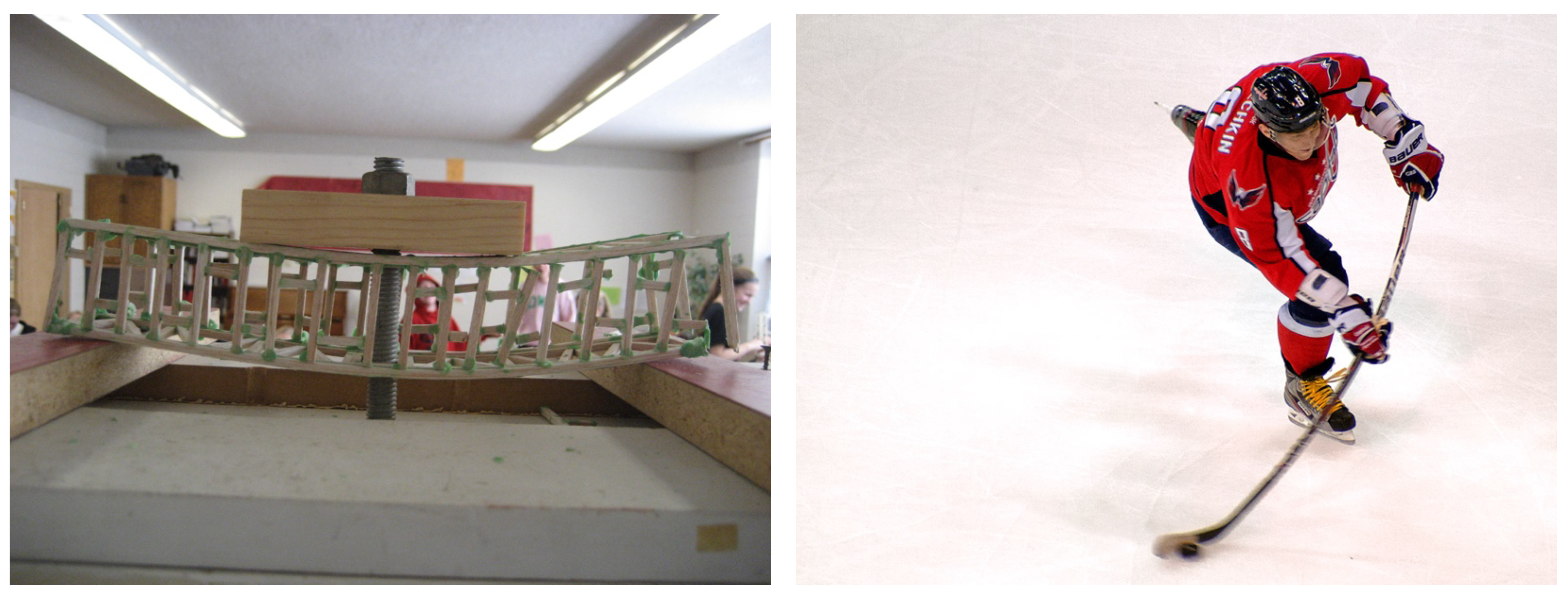
We now know how to calculate both the bending stress (Chapter 9) and shear stress (Chapter 10) in a beam. This chapter considers the deformation of a beam subjected to bending and shear stresses. Under load, beams deflect from their original position (Figure 11.1). Some amount of deflection is unavoidable, but it is usually desirable to limit deflection as much as possible. Although deflection often pose no safety risk (unless the allowable stress of the beam is also exceeded), too much deflection can render a beam unfit for purpose.

Figure 11.1: A model bridge showing severe deflection along its span (left). Although the bridge hasn’t broken, there is too much deflection for the application. The deflection in a hockey stick during a shot (right). In this application the deflection is helpful as it stores and releases energy during the shot.

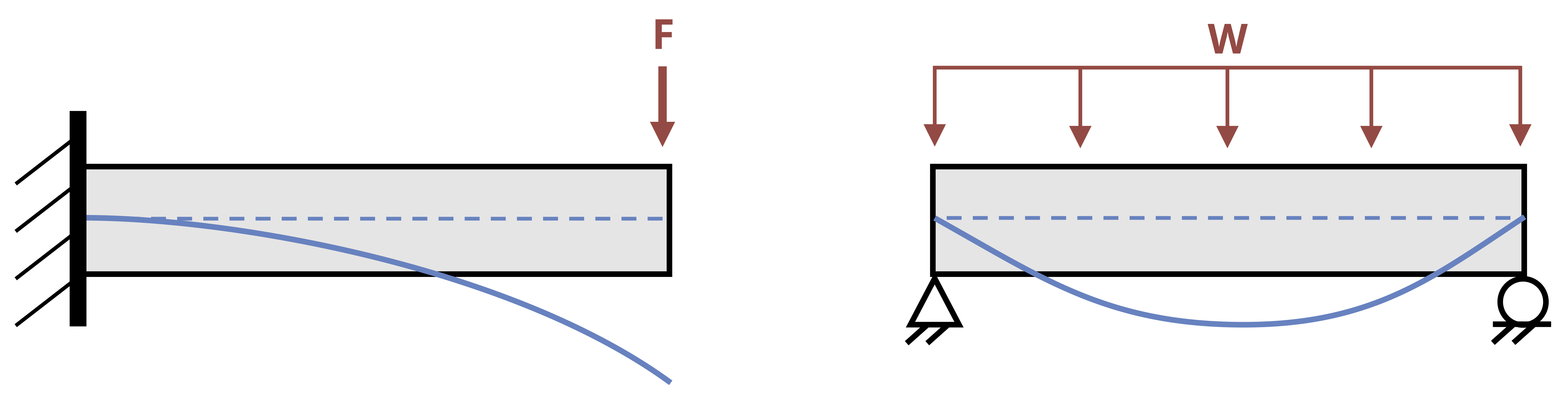
The deflected shape of the beam is known as the elastic curve (Figure 11.2). Exaggerated sketches of the elastic curve provide a quick visual reference of how the beam will deflect and can be used to check that our numerical answers are realistic.

Figure 11.2: Two example beams showing the undeflected position of the centerline (dotted line) and the deflected position (elastic curve) of the beam (solid line).

Section 5.3 showed us how to calculate deformation due to axial load \(\left(\Delta L=\frac{F L}{A E}\right)\). Section 6.2 showed us how to calculate deformation due to torsional load \(\left(\varnothing=\frac{T L}{J G}\right)\). Recall that both types of deformation depend on these elements:

• Applied/internal load (F, T)

• Length of the object (L)

• Cross-section geometry (A, J)

• Material properties (E, G)

It is probably unsurprising, then, that beam deflection also depends on these four elements.

This chapter introduces two common techniques for calculating deflection: the method of integration (Section 11.1 and Section 11.2) and the method of superposition (Section 11.3).

Being able to calculate deflection is vitally important because it allows us to predict how much a beam will deflect before we build a structure. Additionally, being able to calculate deflection will help us solve some more statically indeterminate problems (Section 11.4).

Finally, Section 11.5 enables us to build on our beam design work of Section 9.2 by expanding the specifications to include limitations on shear stress and deflection as well as bending stress.

11.1 Integration of the Moment Equation

Click to expand

We’ll begin by deriving an equation for calculating the deflection at any point in a loaded beam. In Section 9.1 we derived equations relating to bending strain and bending stress.

\[ \varepsilon=-\frac{y}{\rho} \]

\[ \sigma=-\frac{My}{I} \]

Applying Hooke’s law to the strain equation produces

\[ \begin{aligned} \varepsilon=-\frac{y}{\rho}&=\frac{\sigma}{E} \\ \sigma&=-\frac{Ey}{\rho} \end{aligned} \]

Setting the two stress equations equal produces

\[ \frac{E y}{\rho}=\frac{M y}{I} \]

Then rearranging the result yields

\[ \frac{1}{\rho}=\frac{M(x)}{E I} \]

The radius of curvature (ρ) can be related to the deflection (y) by the equation

\[ \frac{1}{\rho}=\frac{\frac{\partial^{2} y}{\partial x^{2}}}{\left[1+\left(\frac{\partial y}{\partial x}\right)^{2}\right]^{\frac{3}{2}}} \]

This equation describes the exact deflection \((y)\) at any distance \((x)\) along the beam for elastic deformations. In most engineering applications the deflection \((y)\) is very small. We can simplify this equation significantly by assuming that the deflection \((y)\) will be small and thus that \(\frac{d y}{d x}\) is very small and \(\left(\frac{d y}{d x}\right)^{2}\) is negligible. This simplifies the equation to

\[ \frac{1}{\rho}=\frac{\frac{\partial^{2} y}{\partial x^{2}}}{[1+0]^{\frac{3}{2}}}=\frac{\partial^{2} y}{\partial x^{2}} \]

Finally, the equation becomes

\[ \frac{1}{\rho}=\frac{\partial^{2} y}{\partial x^{2}}=\frac{M(x)}{E I} \]

To solve for deflection first find an equation for the internal bending moment as a function of \((x)\), using equilibrium just as in Section 7.3 for drawing the bending moment diagram. Then set this equation equal to \(E I \frac{d^{2} y}{d x^{2}}\) and integrate twice.

\[ \boxed{\begin{gathered} M(x)=E I \frac{\partial^{2} y}{\partial x^{2}} \\ \int M(x) d x+C_1=E I \frac{\partial y}{\partial x} \\ \iint M(x) d x+C_1 x+C_2=E I y \end{gathered}} \tag{11.1}\]

In these equations \(y\) represents the deflection of the beam and \(\frac{\partial y}{\partial x}\) represents the slope of the deflected beam. Since the equations are functions of \(x\), we can find the slope and deflection at any point along the beam.

Note that each successive integral introduces a constant of integration that we must solve for. We do this through the use of boundary conditions—that is, points on the beam where we already know the slope and/or deflection. There are two common boundary conditions for our applications:

• At any support the deflection \((y)\) is zero.

• At a fixed support the slope \(\left(\frac{\partial y}{\partial x}\right)\) is zero.

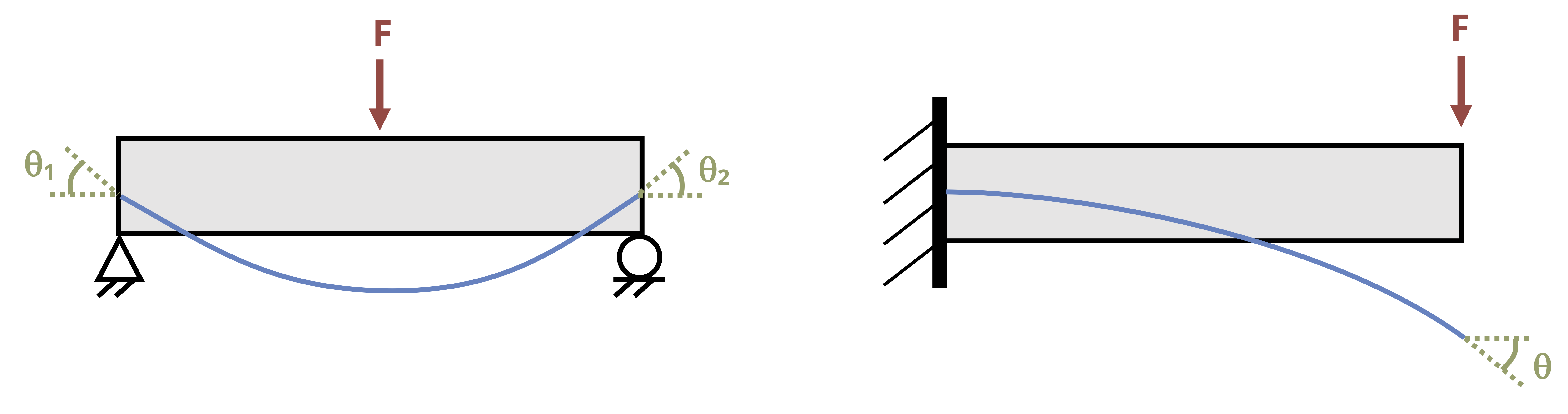
Figure 11.3 illustrates these boundary conditions. Once the constants of integration are known, we can define equations for the slope and deflection of the beam in terms of distance \((x)\) along the beam and calculate the slope and deflection at any value of \(x\). Example 11.1 and Example 11.2 show this process applied to a simply supported beam and a cantilever beam respectively.

Figure 11.3: At pin and roller supports the deflection is zero but the slope is not. At a fixed support both the slope and deflection are zero. A statically determinate beam in equilibrium always has two boundary conditions.

TipExample 11.1

Example 11.1  

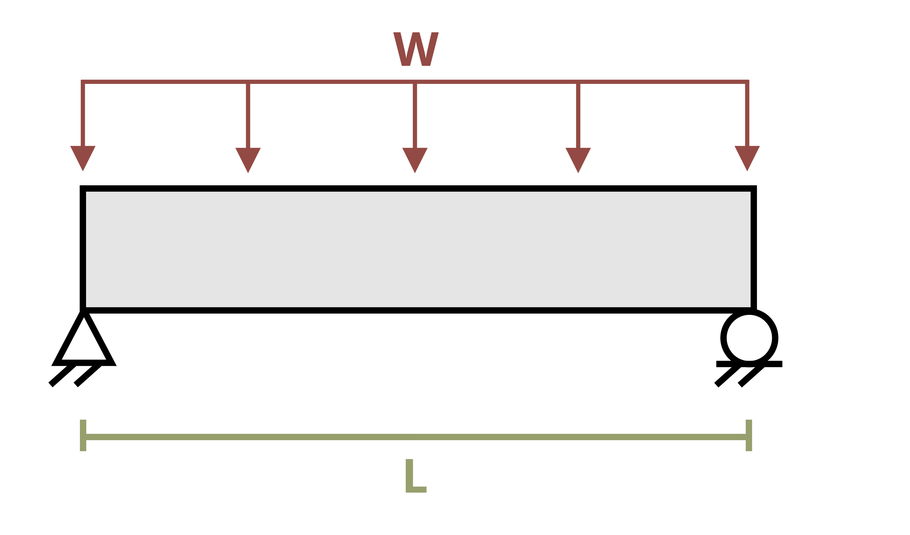
A simply supported beam of length L = 10 m is subjected to a uniform distributed load of w = 20 kN/m.

Determine the equation of the elastic curve and use this to find the deflection of the beam at the midpoint, x = 5 m. Assume E = 200 GPa and I = 350 x 10⁶ mm⁴.

TipSolution

Sketch a free body diagram (FBD) of the beam and use equilibrium equations to solve for the reaction forces at the supports.

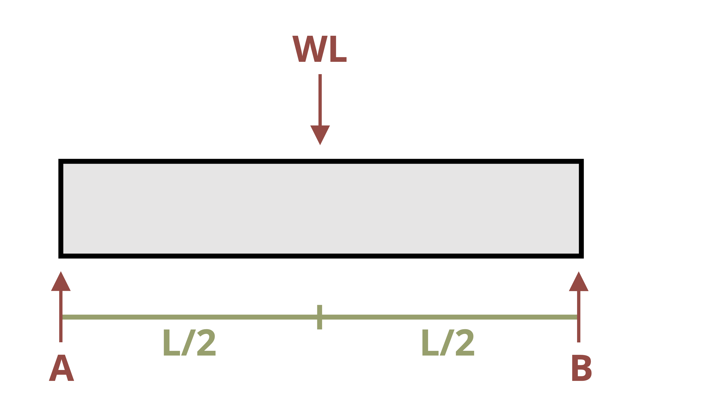
\[ \begin{aligned} & \sum M_A=-wL\left(\frac{L}{2}\right)+B L=0 \quad \rightarrow \quad B=\frac{wL}{2} \\ & \sum F y= A-wL+\frac{wL}{2}=0 \quad\rightarrow\quad A=\frac{wL}{2} \\ & \end{aligned} \]

Cut a cross-section through the beam at distance x and draw an FBD of everything to the left of the cut, including the internal loads. Use equilibrium to determine an equation for the internal bending moment, M, as a function of x.

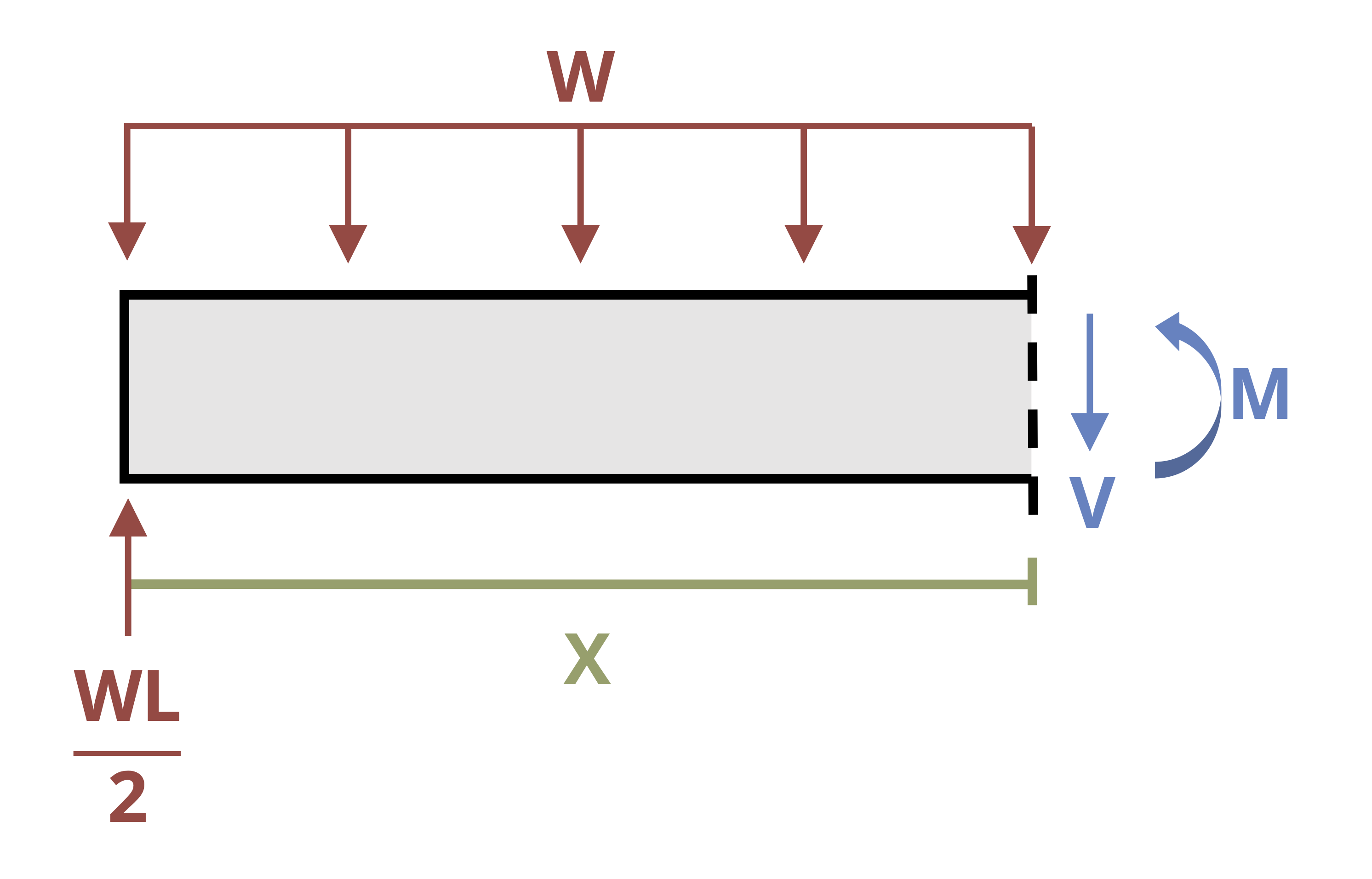
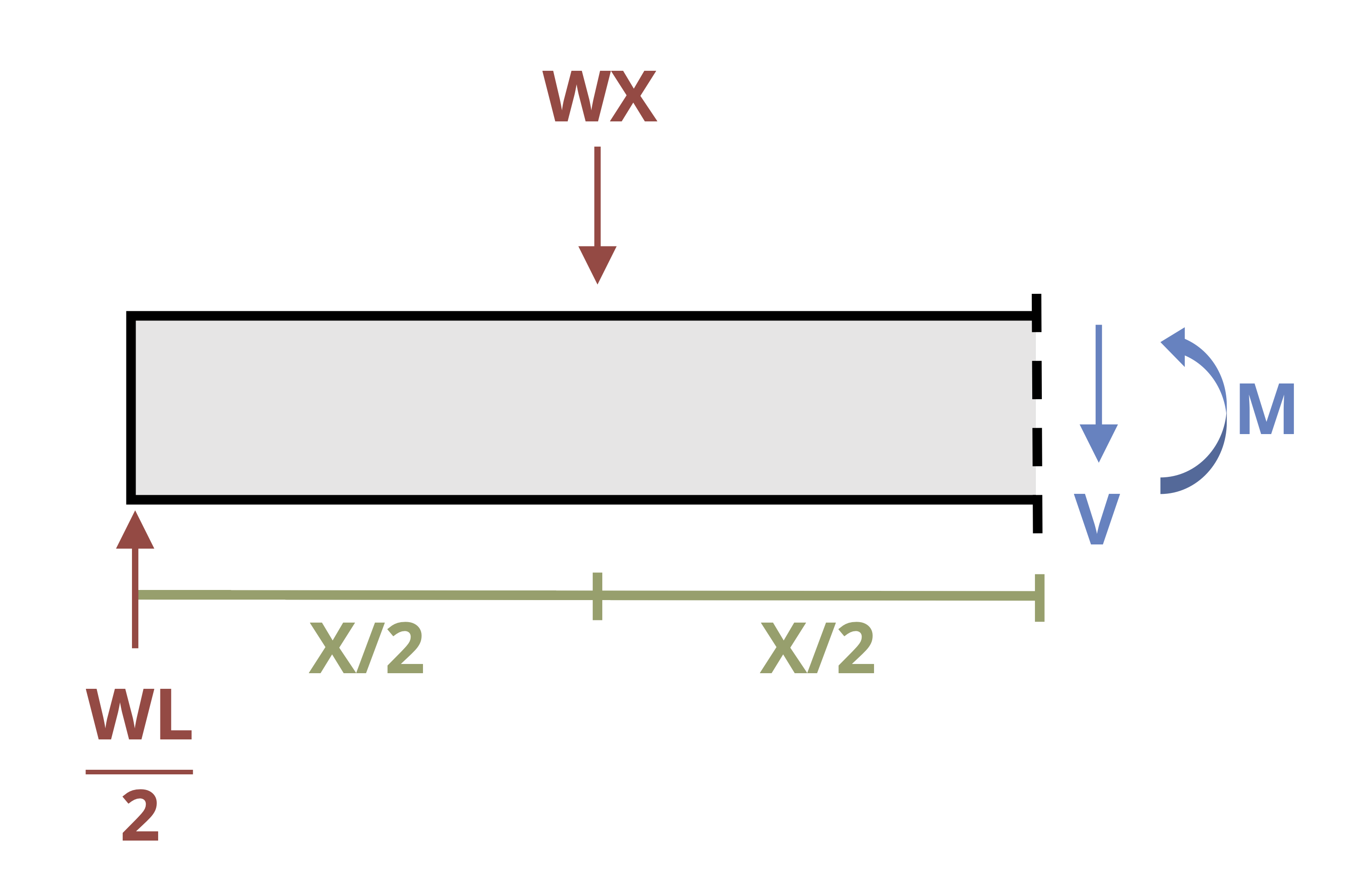
\[ \begin{gathered} \sum M_x= M+w x\left(\frac{x}{2}\right)-\frac{w L}{2}(x)=0 \\ M =\frac{w L x}{2}-\frac{w x^2}{2}=E I \frac{\partial^2 y}{\partial x^2}\end{gathered} \]

Integrate this equation twice.

\[ \begin{aligned} & \frac{w L x^2}{4}-\frac{w x^3}{6}+c_1=E I \frac{\partial y}{\partial x} \\ & \frac{w L x^3}{12}-\frac{w x^4}{24}+c_1 x+c_2=E I y\end{aligned} \]

Apply boundary conditions at the supports.

\[ \begin{aligned} \text { At } x=0, y=0 \quad\rightarrow\quad &C_2=0 \\ \text { At } x=L, y=0 \quad\rightarrow\quad &\frac{w L(L)^3}{12}-\frac{w(L)^4}{24}+C_1 L=0 \\ & C_1=\frac{w L^3}{24}-\frac{wL^3}{12}=-\frac{w L^3}{24}\end{aligned} \]

Substitute these constants into the deflection equation and rearrange.

\[ y=\frac{1}{E I}\left[\frac{w L x^3}{12}-\frac{w x^4}{24}-\frac{wL^3}{24} x\right] \]

Substitute in the given values for and solve this equation at the midpoint (x = 5m).

\[ \begin{aligned} & y=\frac{1}{200 \times 10^9~\frac{N}{m^2}*350 \times 10^{-6}{~m}^4}\left[\frac{20,000~\frac{N}{m}*10{~m}*(5{~m})^3}{12}-\\ \frac{20,000~\frac{N}{m}*(5{~m})^4}{24}-\frac{20,000\frac{N}{m}*(10~{m})^3*5{~m}}{24}\right] \\ & y=-0.0372{~m} \\ & y=-37.2{~mm} \end{aligned} \]

TipExample 11.2

Example 11.2  

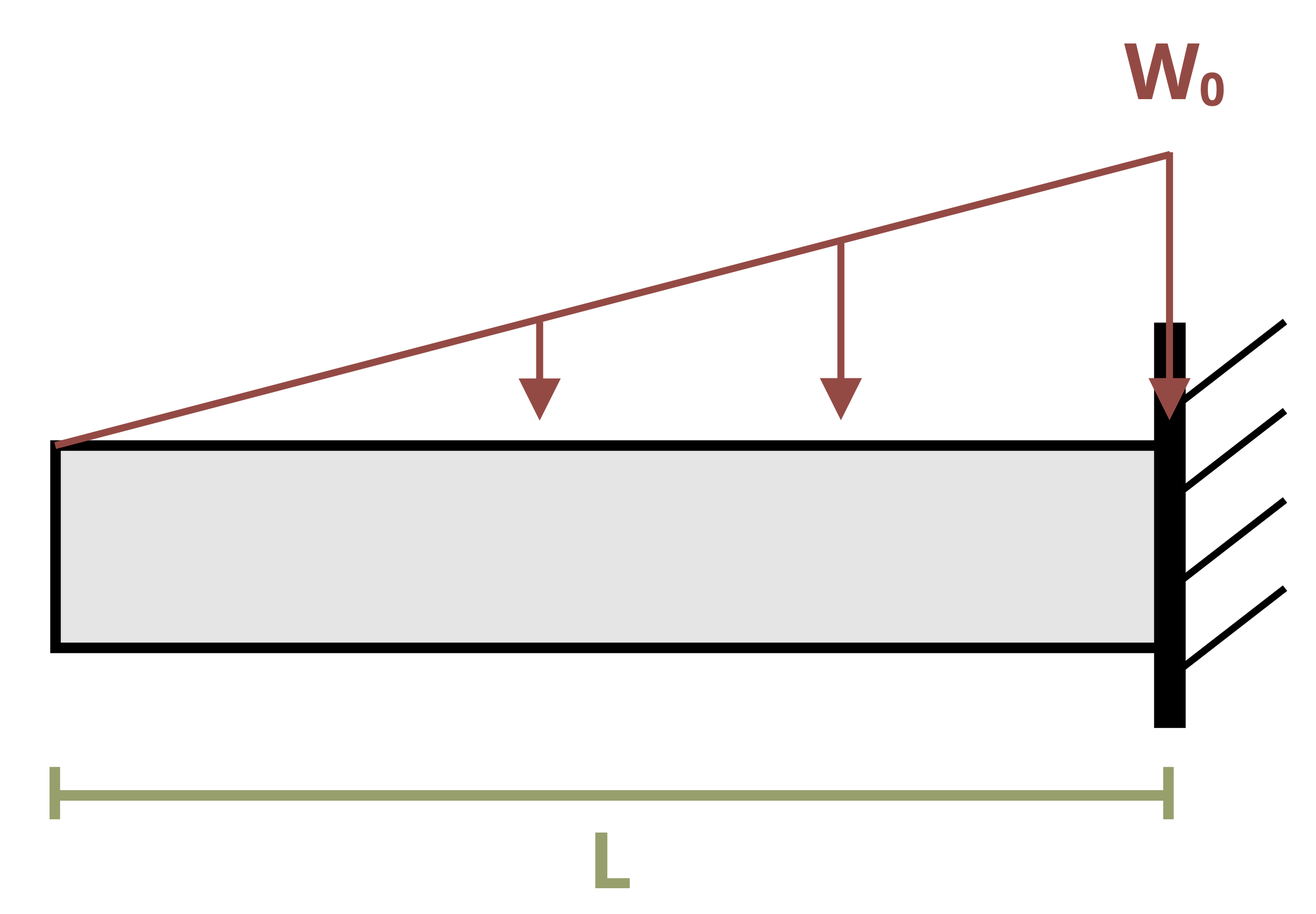
A cantilever beam of length L = 8 ft is subjected to a linear distributed load where w₀ = 30 kip/ft.

Determine the equation of the elastic curve and use this to find the deflection of the beam at the free end. Assume E = 29 x 10⁶ psi and I = 375 in.⁴.

TipSolution

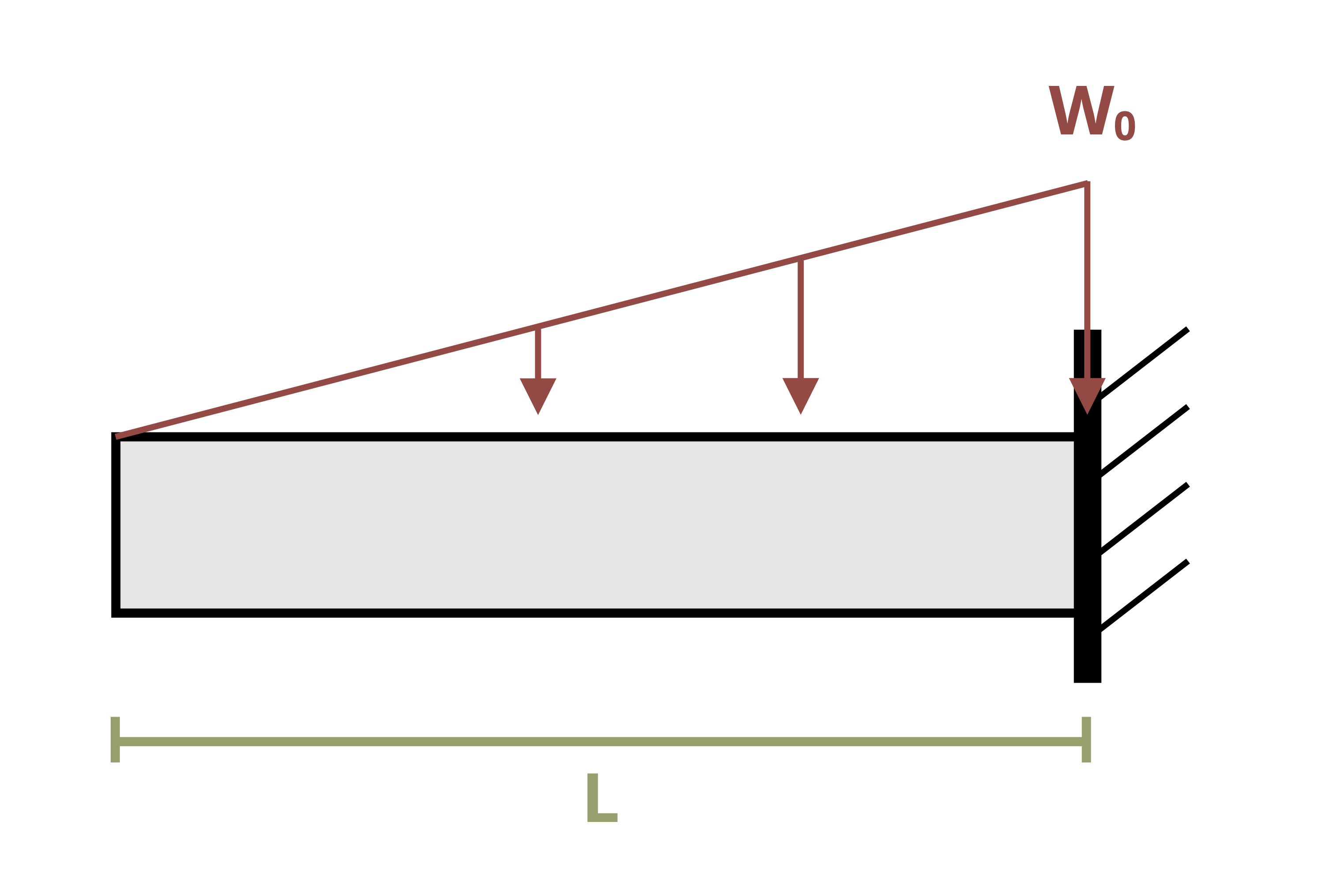
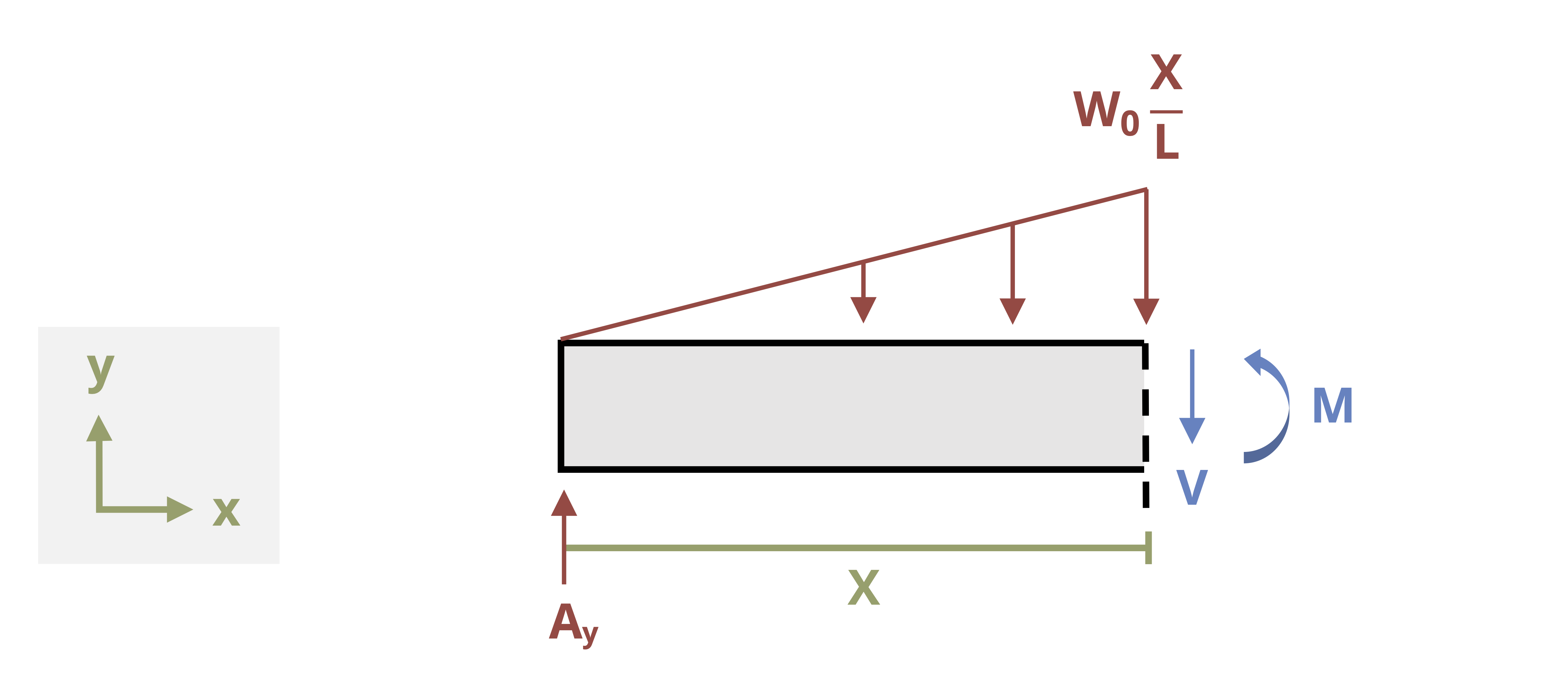
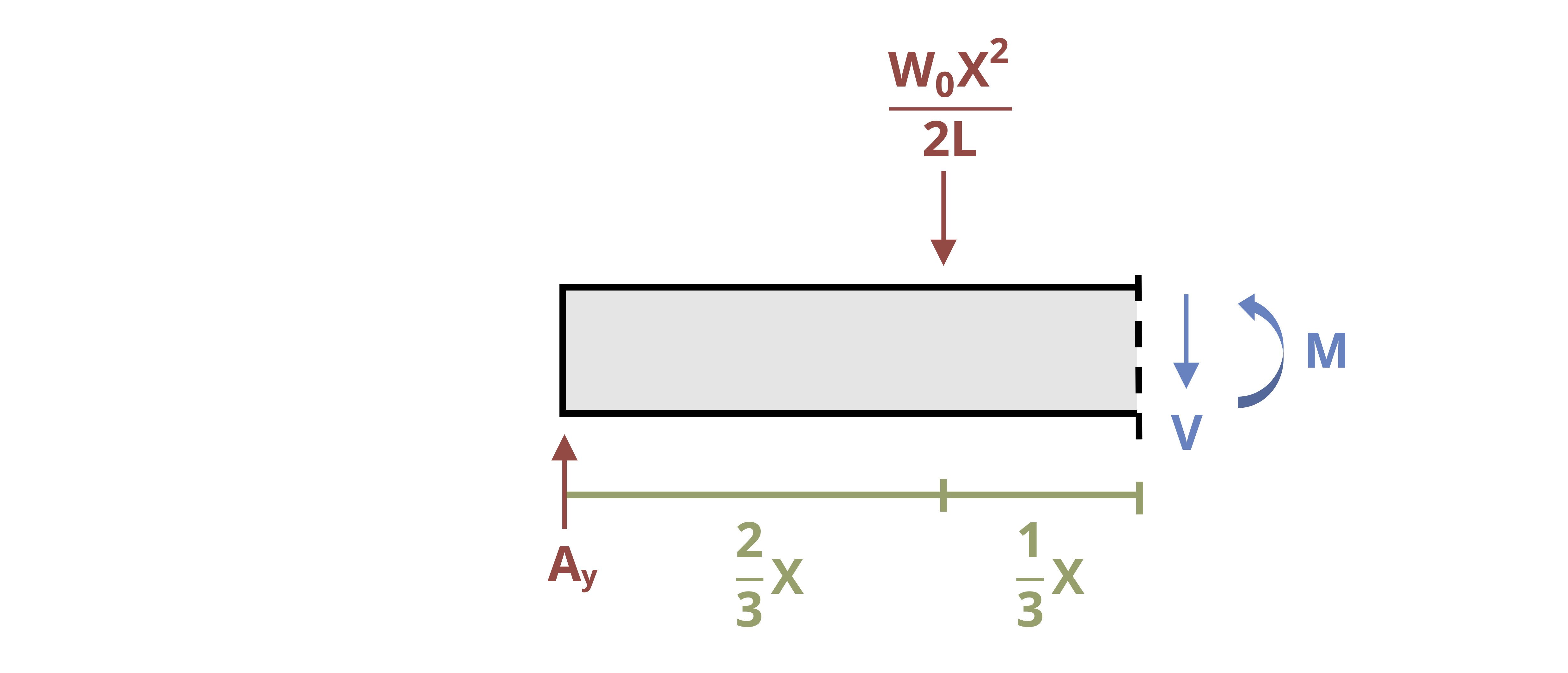
Cut a cross-section through the beam at distance x and draw an FBD of everything to the left of the cut, including the internal loads. This diagram omits the reactions at the fixed support, so there’s no need to solve for these first.

Use equilibrium to determine an equation for the internal bending moment, M, as a function of x. Then integrate this equation twice.

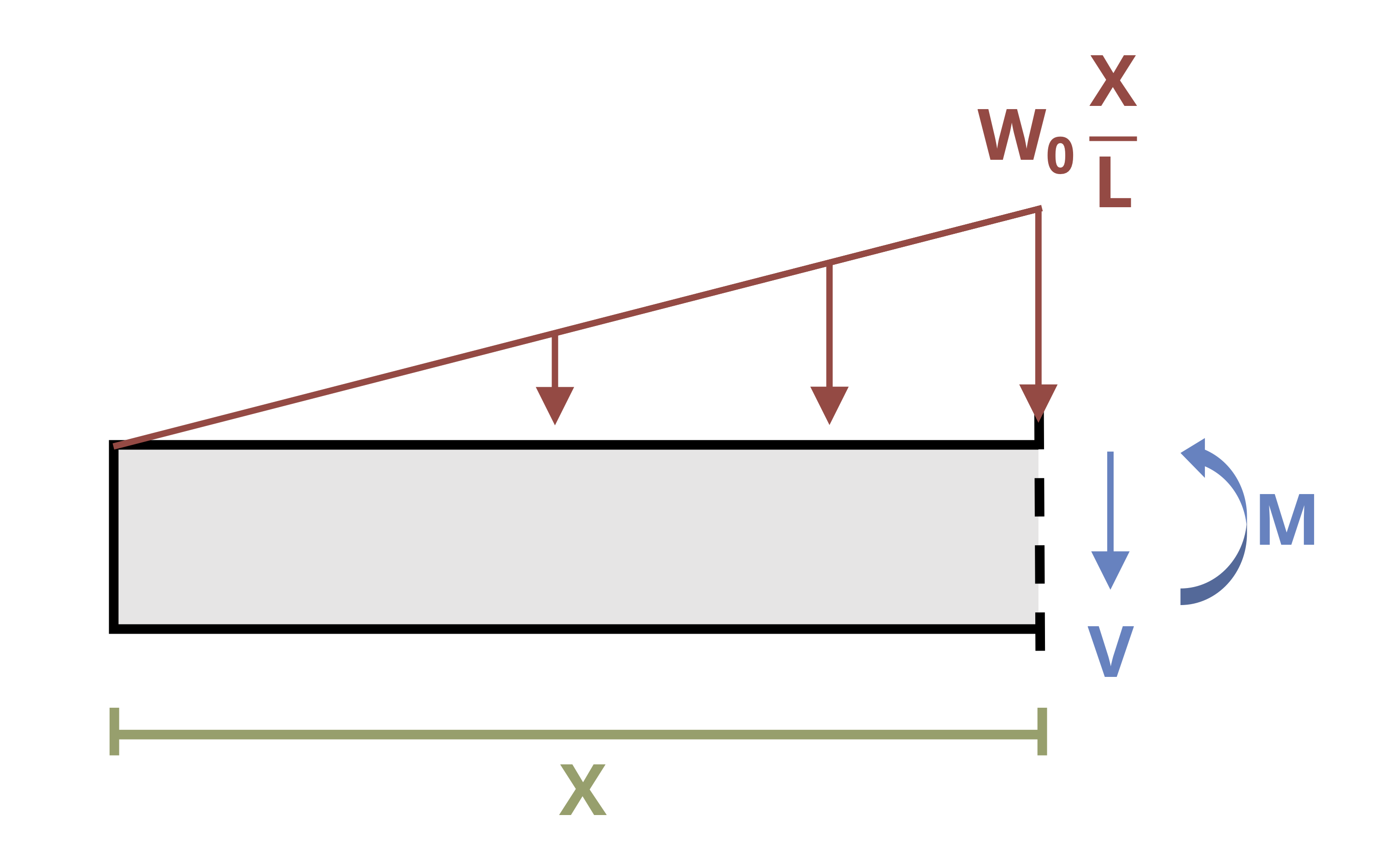
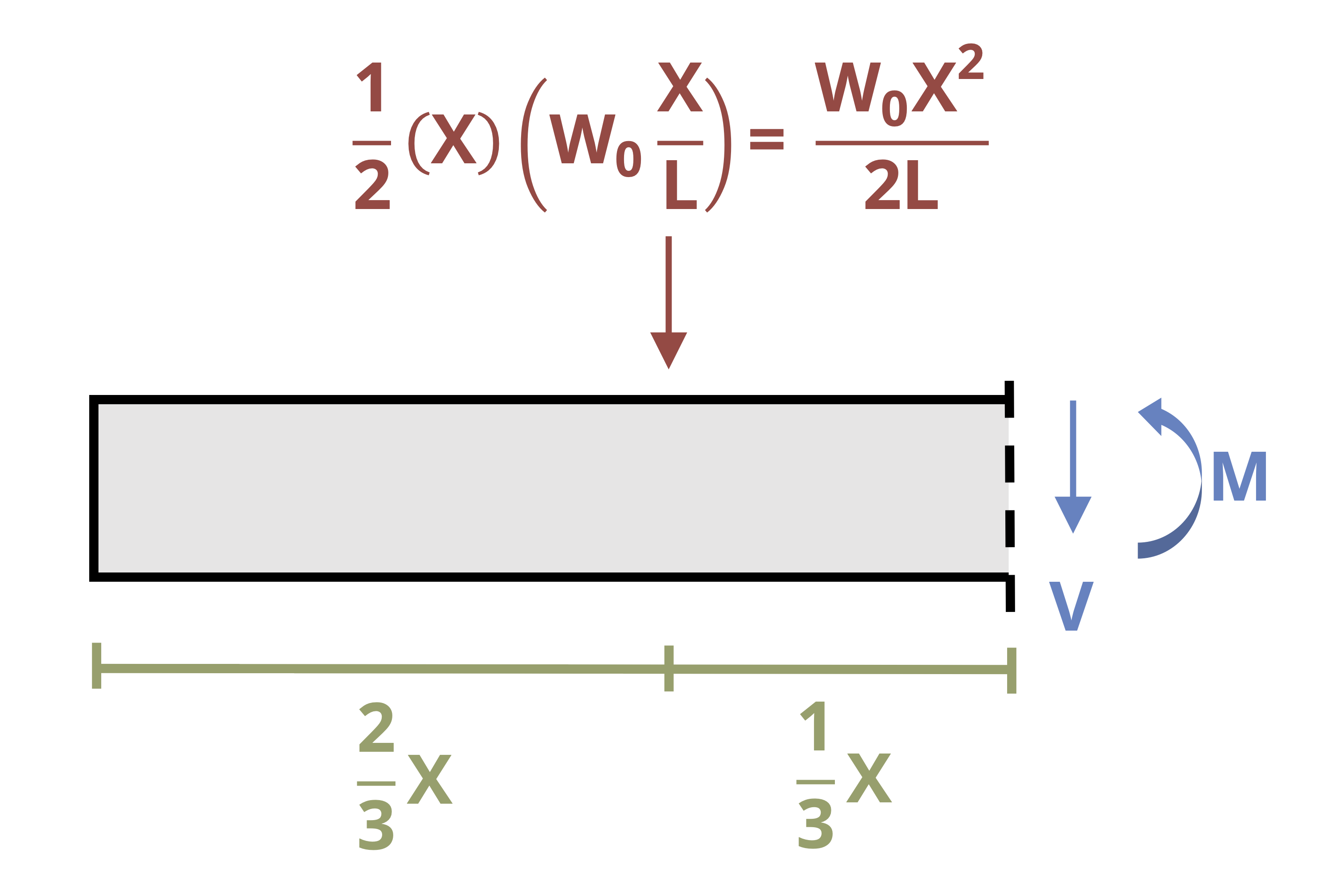
\[ \begin{aligned} \sum M_x=&~M+\frac{w_0 x^2}{2 L}\left(\frac{x}{3}\right)=0 \\ M&=-\frac{w_0 x^3}{6 L}=E I \frac{\partial^2 y}{\partial x^2} \\ \int M~dx&=-\frac{w_0 x^4}{24 L}+C_1=E I \frac{\partial y}{\partial x} \\ \int\int M~dx&=-\frac{w_0 x^5}{120 L}+C_1 x+C_2=EIy \end{aligned} \]

Apply boundary conditions at the fixed support.

\[ \begin{aligned} \text { At } x=L, \frac{\partial y}{\partial x}=0 \quad \rightarrow \quad -~&\frac{w_0 L^4}{24 L}+C_1=0\\ C_1&=\frac{w_0 L^3}{24}\\ \\ \text { At } x=L, y=0 \quad \rightarrow \quad -~&\frac{w_0 L^5}{120 L}+\frac{w_0 L^3}{24}(L)+C_2=0\\ C_2&=\frac{w_0 L^4}{120}-\frac{w_0 L^4}{24}\\ &=-\frac{4 w_0 L^4}{120}\\ &=-\frac{w_0 L^4}{30} \end{aligned} \]

Substitute these constants into the deflection equation and rearrange.

\[ y=\frac{1}{E I}\left[-\frac{w_0 x^5}{120L}+\frac{w_0 L^3}{24} x-\frac{w_0 L^4}{30}\right] \]

Substitute in the given values and solve this equation at the free end (x = 0). Remember to convert feet to inches in both the distributed load and the length.

\[ \begin{aligned} & y=\frac{1}{29 \times 10^6~\frac{lb}{in.^2}*375{~in.^4}} \left[-\frac{\frac{30,000\frac{lb}{ft}}{12~\frac{in.}{ft}}*(8{~ft}*12~\frac{in.}{ft})^4}{30}\right] \\ & y=- 0.651{~in.}\end{aligned} \]

These examples have single continuous loads. If the loading is discontinuous, however, we must modify our approach because no single moment equation can describe the entire beam. Section 7.3 showed that when drawing shear force and bending moment diagrams we can find a different equation for the internal bending moment in each loading region (i.e., a piecewise function over the length of the beam). This requires finding separate moment equations for each loading region and integrating each separately. Do this each time the loading changes, considering

• Both sides of a concentrated load

• A distributed load that begins or ends

This text covers deflection of beams made of a single material with uniform cross-sections (i.e., where elastic modulus, E, and second moment of area, I, remain constant). In practice, changes in E and I necessitate additional separate equations for each change.

Figure 11.4 shows a beam with two loading regions. Fully describing the deflection in this beam requires us to determine two internal bending moment equations—one in segment AB and one in segment BC. Each equation must be integrated twice, thereby introducing four constants of integration. Although two of these can be determined by using boundary conditions, we must determine the remaining two by using continuity conditions.

Figure 11.4: The loading on the simply supported beam is different in segment AB than in segment BC. Each segment has its own bending moment equation that must be found and integrated.

Equation set 1 describes the internal moment, slope, and deflection of the beam from point A to point B, and equation set 2 describes the internal moment, slope, and deflection from point B to point C. Note that both sets of equations describe point B, where the loading changes. They must therefore return the same results at point B. So we can say that

\[ \begin{aligned} \left(\frac{\partial y}{\partial x}\right)_{1} & =\left(\frac{\partial y}{\partial x}\right)_{2} \\ y_{1} & =y_{2} \end{aligned} \]

See Example 11.3 for the full solution for this beam.

TipExample 11.3

Example 11.3  

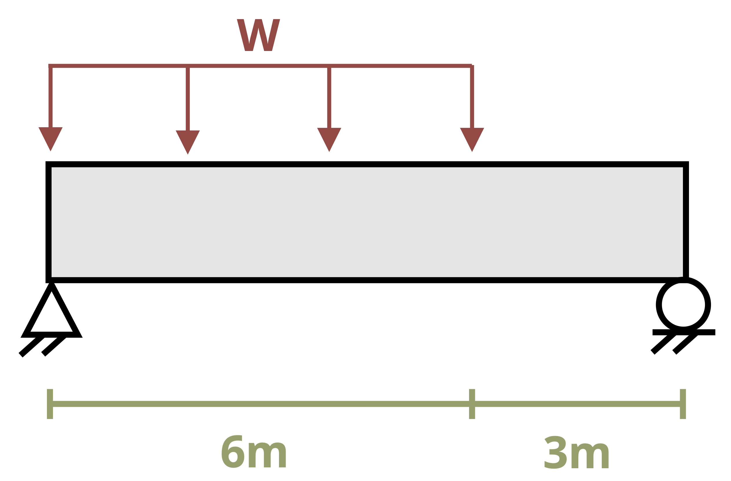
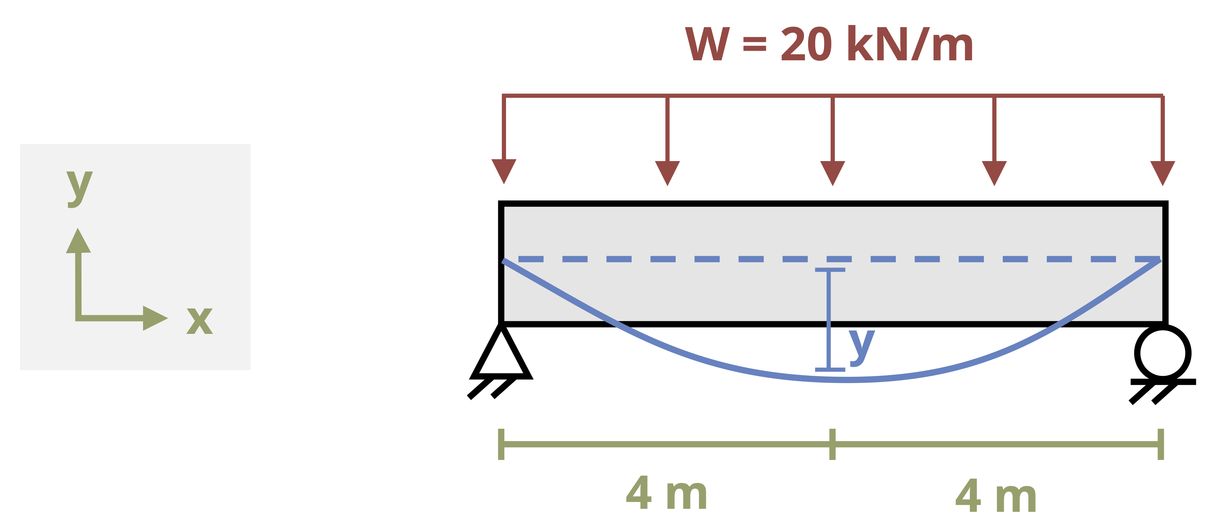
A simply supported beam is subjected to a distributed load of w = 20 kN/m as shown.

Determine the equations of the elastic curve between 0 ≤ x ≤ 6 m and between 6 m ≤ x ≤ 9 m.

Then determine the deflection at x = 5 m. Assume E = 200 GPa and I = 394 x 10⁶ mm⁴.

TipSolution

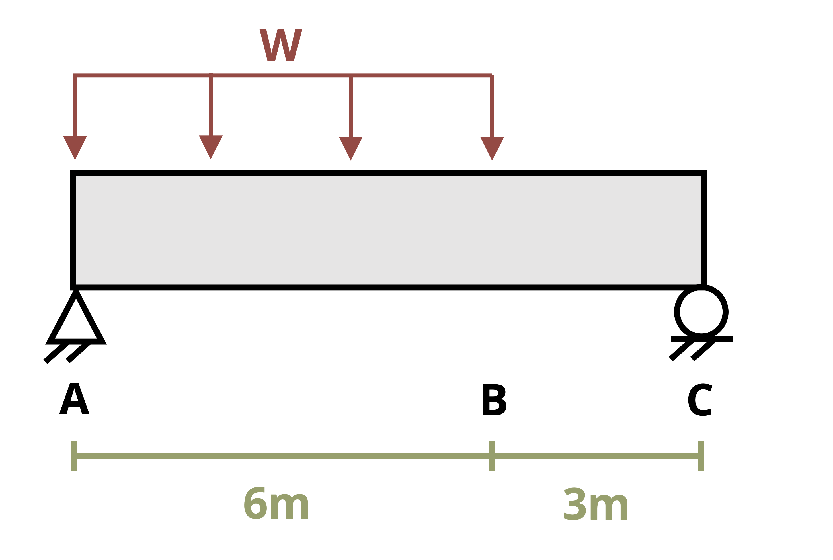
Sketch an FBD of the beam and use equilibrium equations to solve for the reaction forces at the supports.

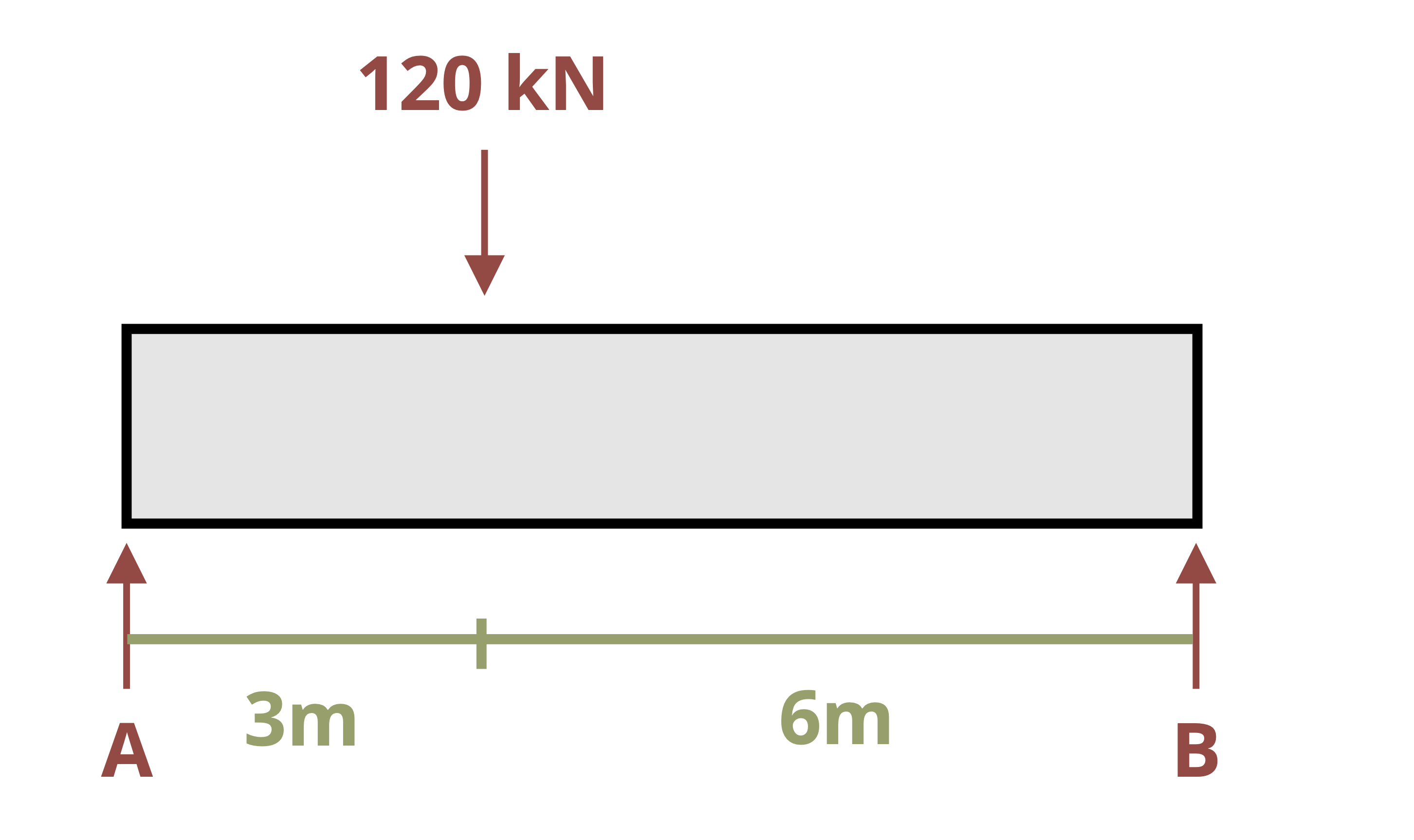
\[ \begin{aligned} & \sum M_A=(120{~kN}*3{~m})+(B*9{~m})=0 \quad \rightarrow \quad B=40{~kN} \\ & \sum F y=-120{~kN}+40{~kN}=0 \quad \rightarrow \quad A=80{~kN} \end{aligned} \]

Cut a cross-section in the first loading region at distance x₁. Draw an FBD of everything to the left of this cut, including the internal loads. Use equilibrium to determine an equation for the internal bending moment, M₁, as a function of x₁. Then integrate this equation twice.

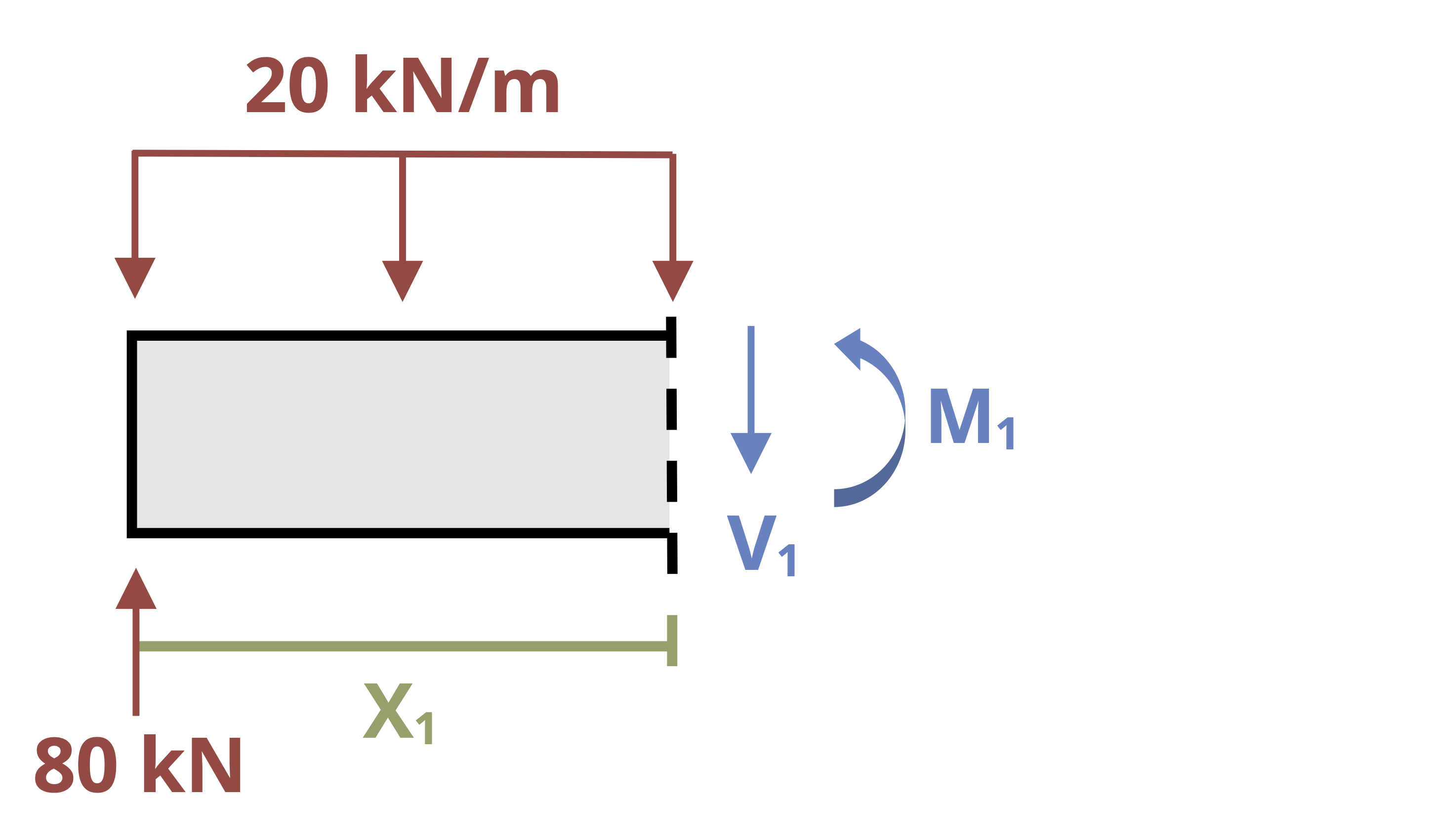
\[ \begin{aligned} \sum M_x=&~M_1+20 x_1\left(\frac{x_1}{2}\right)-80 x_1=0 \\ M_1&=80 x_1-10 x_1^2=E I \frac{\partial^2 y_1}{\partial x_1^2} \\ \int M_1~dx&=\frac{80 x_1^2}{2}-\frac{10 x_1^3}{3}+c_1=E I \frac{\partial y_1}{\partial x_1} \\ \int\int M_1~dx&=\frac{80 x_1^3}{6}-\frac{10 x_1^4}{12}+c_1 x_1+c_2=E I y_1 \end{aligned} \]

These equations are valid from 0 ≤ x₁ ≤ 6 m.

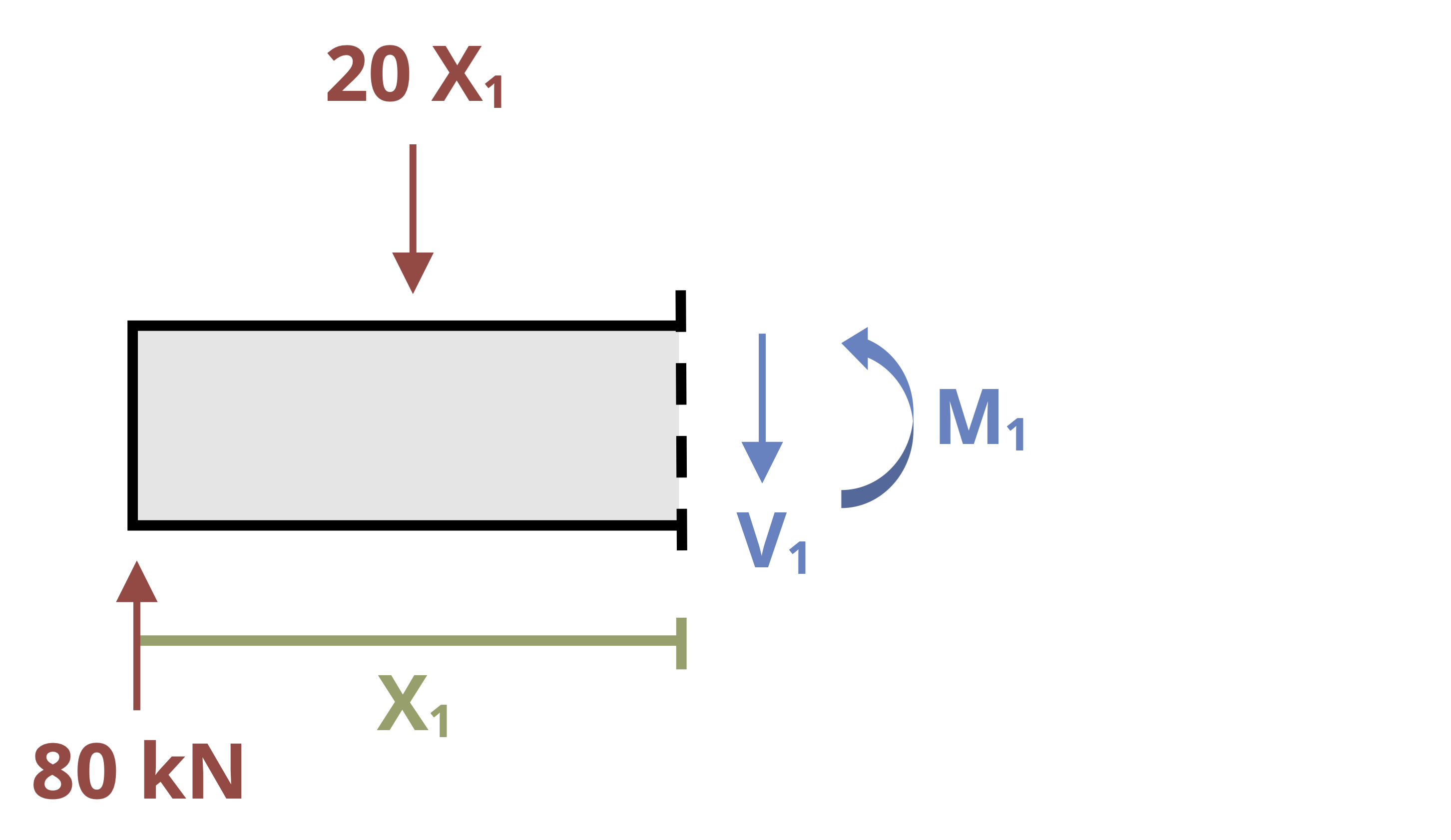
Set these equations aside and cut a cross-section in the second loading region at distance x₂. Draw an FBD of everything to the left of this cut, including the internal loads.

Use equilibrium to determine an equation for the internal bending moment, M₂, as a function of x₂. Then integrate this equation twice.

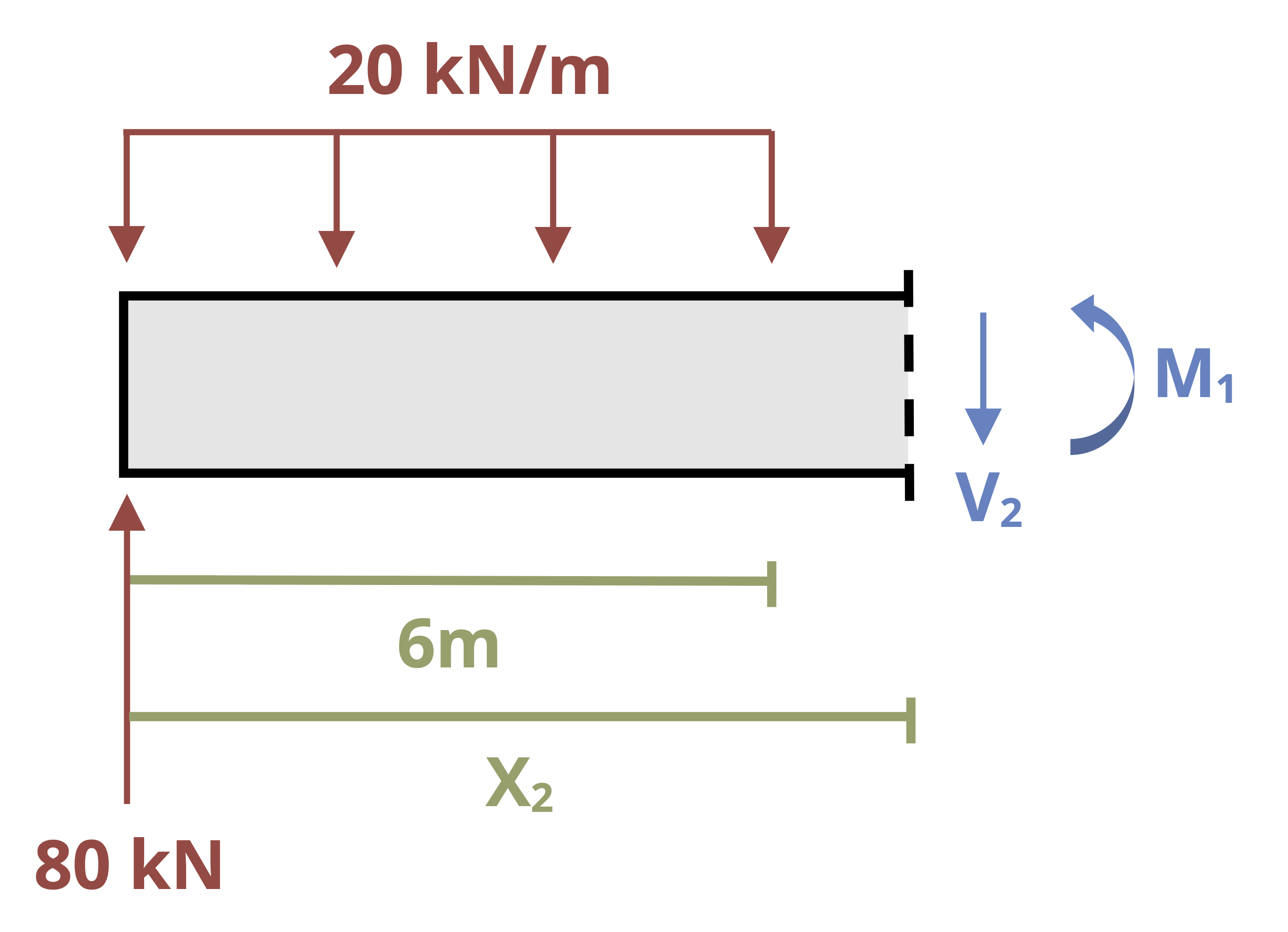
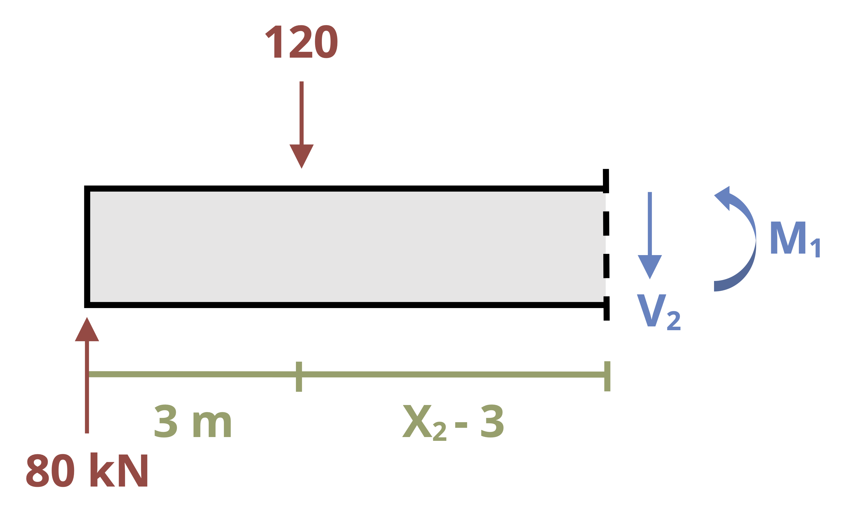
\[ \begin{aligned} \sum M_x=&~ M_2+120\left(x_2-3\right)-80 x_2=0 \\ M_2&=80 x_2-120 x_2+360 \\ M_2&=360-40 x_2=E I \frac{\partial^2 y_2}{\partial x_2^2} \\ \int M_2~dx&=360 x_2-\frac{40 x_2^2}{2}+c_3=E I \frac{\partial y_2}{\partial x_2} \\ \int\int M_2~dx&=\frac{360 x_2^2}{2}-\frac{40 x_2^3}{6}+c_3 x_3+c_4 =E I y_2 \end{aligned} \]

These equations are valid from 6 m ≤ x₂ ≤ 9 m.

Apply bounding conditions at the supports. One support is in loading region 1 and the other is in region 2. Be careful to use the appropriate deflection equation when applying the boundary conditions.

\[ \begin{aligned} \text { At } x_1=0, y_1=0 \quad \rightarrow \quad &c_2=0 \\ \text { At } x_2=9, y_2=0 \quad \rightarrow \quad &\frac{360(9)^2}{2}-\frac{40(4)^3}{6}+c_3(9) +C_4=0 \\ & c_4=-9 c_3-9,720\end{aligned} \]

Apply continuity conditions at the point where the loading changes (x₁ = x₂ = 6 m).

\[ \begin{gathered} \text { At } x_1=x_2=6 \mathrm{~m}, \frac{\partial y_1}{\partial x_1}=\frac{\partial y_2}{\partial x_2} \\ \frac{80(6)^2}{2}-\frac{10(6)^3}{3}+c_1=360(6)-\frac{40(6)^2}{2}+c_3 \\ 1,440-720+c_1=2,160-720+c_3 \\ C_1=720+C_3 \\ \\ \text { At } x_1=x_2=6 \mathrm{~m}, y_1=y_2 \\ \frac{80(6)^3}{6}-\frac{10(6)^4}{12}+c_1(6)=\frac{360(6)^2}{2} - \frac{40(6)^3}{6}+c_3(6) +C_4 \\ 2,880-1,080+6 C_1=6,480-1,440+6 C_3+C_4 \\ 1,800+6 C_1=5,040+6 C_3+C_4 \\\end{gathered} \]

Substitute in C₄ = -9C₃ - 9,720 and C₁ = 720 + C₃.

\[ \begin{gathered} 1,800+6\left(720+c_3\right)=5,040+6 c_3+c_4 \\ 1,800+4,320+6 c_3=5,040+6 c_3+c_4 \\ 6,120-5,040=c_4 \\ c_4=1,080 \\\\ c_4=-9 c_3-4,720 \\ c_3=\frac{-1,080-9,720}{9} \\ c_3=-1,200 \\\\ c_1=720+c_3=720-1,200 \\ c_1=-480 \end{gathered} \]

Substitute constants into deflection equations.

\[ \begin{aligned}y_1 & =\frac{1}{E I}\left[\frac{80 x_1^3}{6}-\frac{10 x_1^4}{12}-480 x_1\right] \\y_2 & =\frac{1}{E I}\left[\frac{360 x_2^2}{2}-\frac{40 x_2^3}{6}+1,200 x_3+1,080\right]\end{aligned} \]

Deflection at midpoint occurs when x₁ = 5 m.

\[ \begin{aligned} y_1&=\frac{1}{EI} {\left[\frac{80{~kN}*(5{~m})^3}{6}-\frac{10~\frac{kN}{m}*(5{~m})^4}{12}-480{~kN}\cdot{m^2}*(5{~m})\right] \\ =-\frac{1,254 \times 10^3{~N}\cdot{m}^3}{200 \times 10^9~\frac{N}{m^2}*394 \times 10^{-6}{~m}^4} } \\ y_1 & =-~0.0159{~m} \\ & =-~15.9{~mm} \\ \end{aligned} \]

Note that we are not required to make both cuts from the left to find the internal bending moment. In some cases making one cut from the left and the other from the right may be the easier approach. Consider the beam in Figure 11.5. Given a cut in the region not under the distributed load, an FBD of the left side of the cut shows many more forces than an FBD of the right side.

Figure 11.5: Simple beam showing two options for finding the internal bending moment. Note that the moment equation will be much simpler if we draw the right-hand side of the cut.

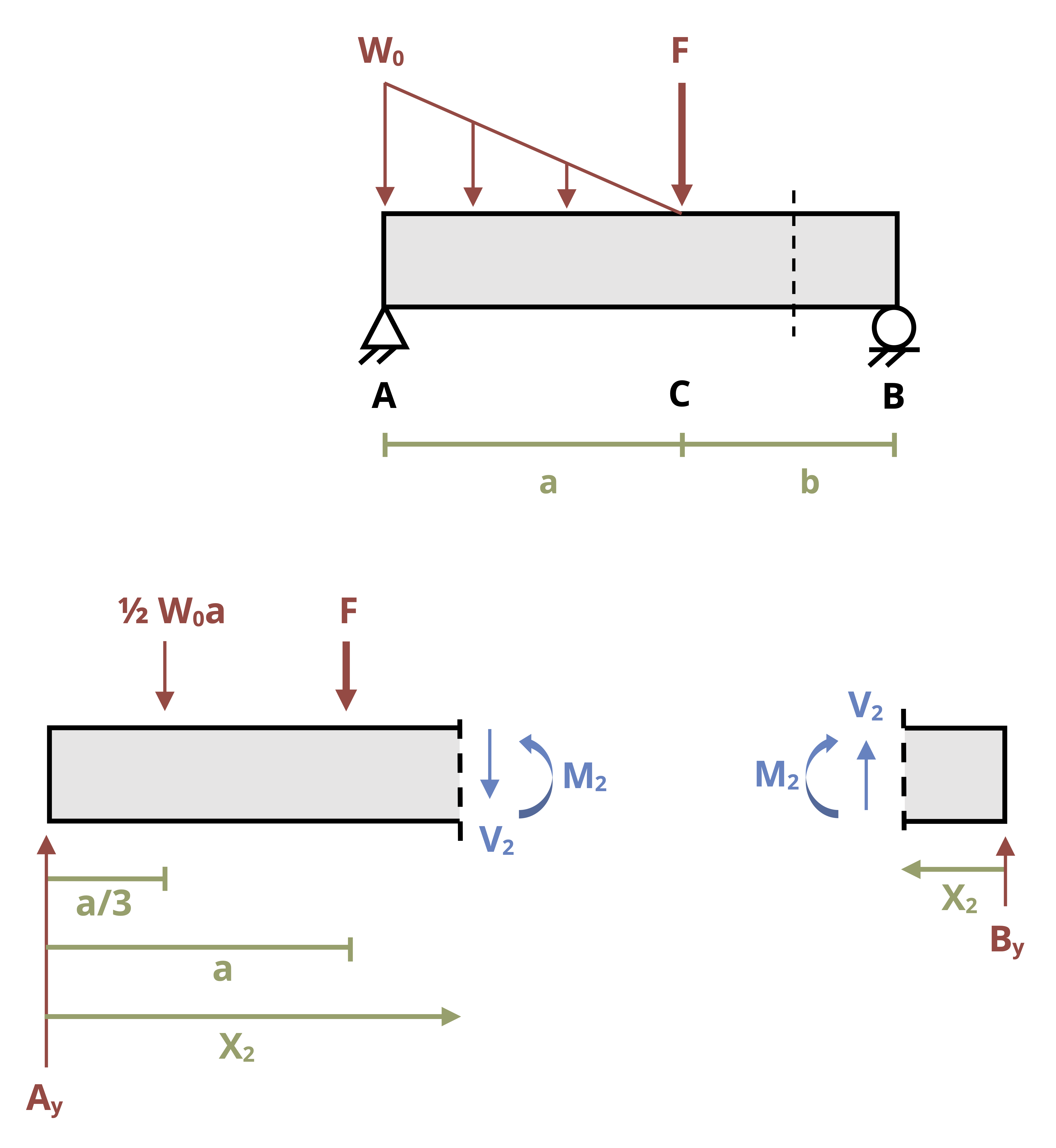
The moment equation is less complex if we draw the right-hand side of the cut rather than the left-hand side. This in turn simplifies the integrations and the math involved in finding the constants of integration.

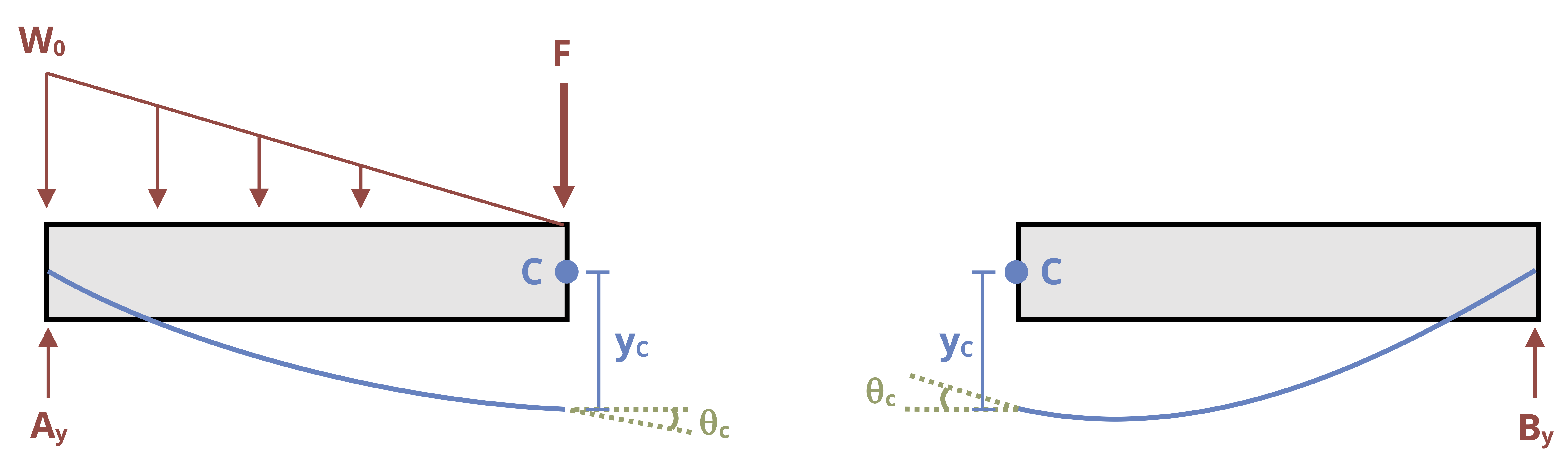
If, however, we do measure distance x₂ from the right, we must make one change to the continuity conditions. Recall that when both cuts are from the left, at point C the slope and deflection calculated from equation 1 must be the same as those calculated from equation 2.

\[ \begin{aligned} \left(\frac{\partial y}{\partial x}\right)_{1} & =\left(\frac{\partial y}{\partial x}\right)_{2} \\ y_{1} & =y_{2} \end{aligned} \]

When distance x₂ is measured from the right, \(y_1 = y_2\) at point C because the deflection is downward whether we measure the horizontal distance from the left or from the right. The magnitude of the slope will also be the same at point C regardless of which equation we use to calculate it. However, the direction of rotation of the slope will change from counterclockwise to clockwise because we have changed the coordinate system (Figure 11.6). Thus our second boundary condition must become

\[ \left(\frac{\partial y}{\partial x}\right)_{1}=-\left(\frac{\partial y}{\partial x}\right)_{2} \]

Figure 11.6: Depending on which side of the cut we draw, the deflection at point C will have the same magnitude and direction. The slope at point C will have the same magnitude but opposite directions if one cut is from the left and the other from the right.

This negative sign is vitally important, and we will not obtain the correct answer if we forget to include it. Example 11.3 has been reworked, this time with one cut made from the right-hand side. Compare this with the previous solution to see the differences.

TipExample 11.3 (reworked)

A simply supported beam is subjected to a distributed load of w = 20 kN/m as shown.

Determine the equation of the elastic curve between 0 ≤ x ≤ 6 m and between 6 m ≤ x ≤ 9 m.

Then determine the deflection at x = 5 m. Assume E = 200 GPa and I = 394 x 10⁶ mm⁴.

TipSolution

Proceed through the first cut as before and find

\[ \begin{aligned} & \frac{80 x_1^2}{2}-\frac{10 x_1^3}{3}+c_1=EI\frac{\partial y_1}{\partial x_1} \\ & \frac{80 x_1^3}{6}-\frac{10 x_1^4}{12}+c_1 x_1+c_2=-EI y_1\end{aligned} \]

Make a second cut from the right hand side. Draw an FBD and use equilibrium to determine an equation for the internal bending moment, M₂, as a function of x₂. Then integrate this equation twice.

\[ \begin{aligned} \sum M_x=&~40 x_2-M_2=0 \\ M_2&=40 x_2=EI\frac{\partial^2 y_2}{\partial x_2^2} \\ \int M_2~dx&=\frac{40 x_2^2}{2}+c_3=EI \frac{\partial y_2}{\partial x_2} \\ \int\int M_2~dx&=\frac{40 x_2^3}{6}+c_3 x_2+c_4=E I y_2 \\ \end{aligned} \]Apply boundary conditions as before, although this time the roller support is at x₂ = 0 since we’re measuring x₂ from the right side.

\[ \begin{aligned} & \text { At } x_1=0, y_1=0 \quad \rightarrow \quad c_2=0 \text { (as before) }\\ & \text { At } x_2=0, y_2=0 \quad \rightarrow \quad c_4=0\end{aligned} \]

Apply continuity conditions at the point where the loading changes (x₁ = 6 m, x₂ = 3 m).

\[ \begin{gathered} \text { At } x_1=6~m,~x_2=3~m,~y_1=y_2\\ \\ \frac{80(6)^3}{6}-\frac{10(6)^4}{12}+ c_1(6)=\frac{40(3)^3}{6}+c_3(3) \\ 2,880-1,080+6 c_1=180+3 c_3 \\ 540+2 c_1=c_3 \\ \\ \text { At } x_1=6~m,~x_2=3~m,~\frac{d y_1}{d x_1}=-\frac{d y_2}{d x_2} \\ \\ \frac{80(6)^2}{2}-\frac{10(6)^3}{3}+c_1=-\frac{40(3)^2}{2}-c_3 \\ 1,440-720+c_1=-180-c_3 \\ 900+c_1=-c_3 \\\end{gathered} \]

Substitute in 540 + 2c₁ = c₃.

\[ \begin{aligned} 540+2 c_1 & =-900-c_1 \\ 3 c_1 & =-1,440 \\ c_1 & =-480 \text { (as before) }\end{aligned} \]

\[ \begin{aligned} & 900-480 =-c_3 \\ & c_3 =-420 \end{aligned} \]

Substitute constants into deflection equations.

\[ \begin{aligned} & y_1=\frac{1}{EI}\left[\frac{80 x_1^3}{6}-\frac{10 x_1^4}{12}-480 x_1\right] \quad \text { (as before) } \\ & y_2=\frac{1}{E I}\left[\frac{40 x_2^3}{6}-420 x_2\right]\end{aligned} \]

Deflection at midpoint occurs when x₁ = 5 m.

\[ \begin{aligned} y_1&=\frac{1}{EI}{\left[\frac{80{~kN}*(5{~m})^3}{6}-\frac{10~\frac{kN}{m}*(5{~m})^4}{12}-480{~kN}\cdot{m}^2*(5{~m})\right] \\ =-\frac{1,254 \times 10^3{~N}\cdot{m}^3}{200 \times 10^9~\frac{N}{m^2}*394 \times 10^{-6}{~m}^4} } \\ y_1 & =~-0.0159{~m} \\ & =-~15.9{~mm} \end{aligned} \]

WarningStep-by-Step: Deflection by Integration of Moment Equation

1. Solve for reaction loads using equilibrium.

2. Cut a cross-section through the beam and find the internal bending moment as a function of x. If the external loading changes, repeat this in each segment of the beam.

3. Set the internal bending moment \(M(x)=E I \frac{d^{2} y}{d x^{2}}\) and integrate twice.

4. Use boundary conditions to determine two constants of integration.

   1. At a fixed support slope \(\left(\frac{\partial y}{\partial x}\right)=0\).
   2. At any support deflection \((\mathrm{y})=0\).

5. In cases with more than one region of load, apply continuity conditions to determine additional constants of integration. At the point where the loading changes find

   1. \(\left(\frac{\partial y_1}{\partial x_1}\right)=\left(\frac{\partial y_2}{\partial x_2}\right)\)

   2. \(y_1=y_2\)

6. Determine the slope and deflection at any value of x as required.

11.2 Integration of the Load Equation

Click to expand

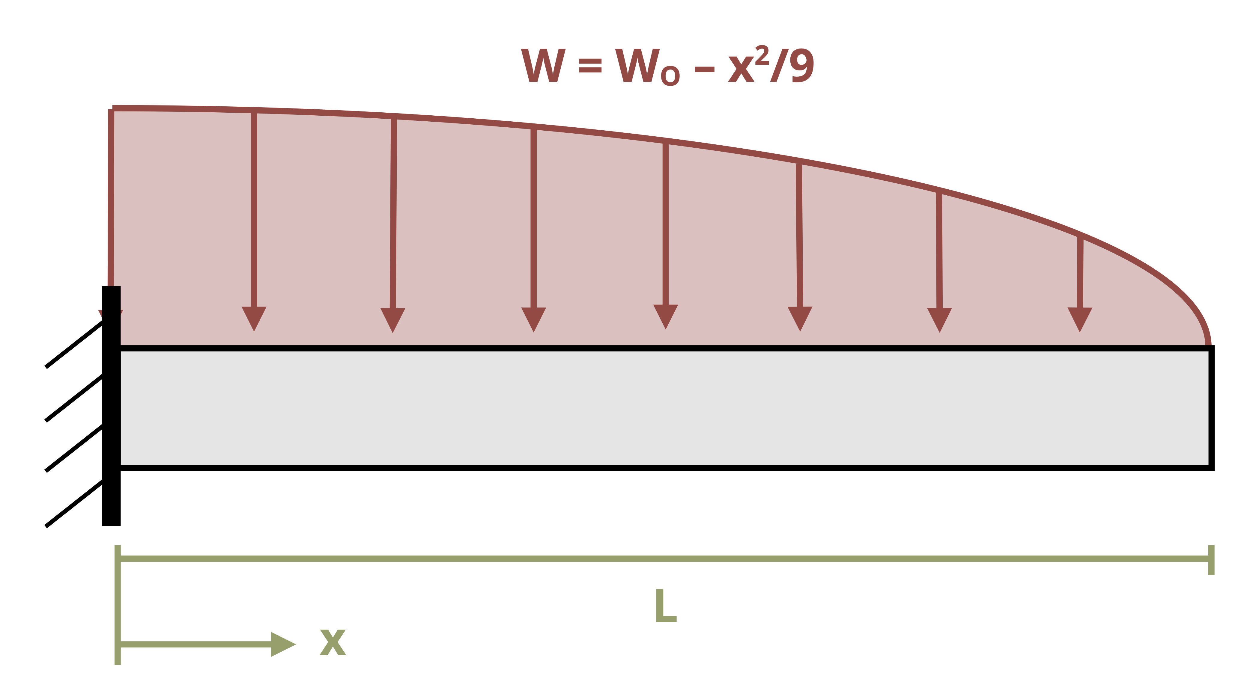
In the previous section we used equilibrium to determine the equation of the internal bending moment and integrated this equation twice. This approach works well for relatively simple loading such as concentrated loads and uniformly or linearly distributed loads. For more complex loads, such as that shown in Figure 11.7, determining the internal bending moment equation in this way can be difficult. However, it’s possible to avoid the need to do so.

Figure 11.7: Complex external loads make it difficult to use equilibrium to determine the internal bending moment equation.

In Section 11.1 we used equilibrium equations to determine the internal bending moment in a beam as a function of x. We related this bending moment to the deflection by

\[ M(x)=E I \frac{\partial ^{2} y}{\partial x^{2}} \]

In Section 7.2 we learned that there is a relationship between the internal bending moment, the internal shear force, and the external load. For an external distributed load, w, we found

\[ V=\int_{0}^{L} w(x) d x \]

\[ M=\int_{0}^{L} V(x) d x \]

We may therefore relate the deflection of a beam not only the internal bending moment but also to the internal shear force and external distributed load through successive integrations. For some loading configurations it can be simpler to integrate the distributed load equation four times instead of finding the equation of the internal bending moment through equilibrium and integrating twice. When taking the simpler approach, remember that loads acting downward (as most loads on beams do) are negative.

\[ \boxed{\begin{aligned} &w(x)=E I \frac{\partial^{4} y}{\partial x^{4}} \\ &V(x)=E I \frac{\partial^{3} y}{\partial x^{3}}=\int w(x)~dx+C_1 \\ &M(x)=E I \frac{\partial^{2} y}{\partial x^{2}}=\int V(x)~dx+C_2 \\ &EI\theta(x)=E I \frac{\partial y}{\partial x}=\int M(x)~dx+C_3 \\ &EIy(x)=\int \theta(x)~dx+C_4 \end{aligned}} \tag{11.2}\]

Note that each successive integral will introduce a new constant of integration. To solve for these constants we must again apply boundary conditions. Now with four constants four boundary conditions are required. Two of these conditions are the same as those in Section 11.1:

• At any support the deflection is 0.

• At a fixed support both slope and deflection are zero.

The other two boundary conditions come from knowing the value of the shear force and bending moment at a point in the beam. Our work in Chapter 7 enables us to find them. Although we can use known values at any point in the beam, it is generally easiest to use the shear force and bending moment at x = 0. Note the two conditions at this point:

• The shear force will be equal to the applied force (including a force applied by a support) if there is one, or zero otherwise.

• The bending moment will be equal to the applied moment (including a moment applied by a fixed support) if there is one, or zero otherwise.

Example 11.4 demonstrates of how to find the deflection of a beam by integrating the load equation. Although this method can be used for any beam, it is best applied to beams with a single continuous distributed load acting over the length of the beam. Beams with discontinuous loading require integration of multiple load equations.

TipExample 11.4

Example 11.4  

The cantilever beam from Example 11.2 is repeated here. Length L = 8 ft is subjected to a linear distributed load where w₀ = 30 kip/ft.

Determine the equation of the elastic curve and use this to find the deflection of the beam at the free end.

TipSolution

First define the equation of the load, which increases linearly from zero to w₀.

\[ \omega=-\omega_0 \frac{x}{L}=E I \frac{\partial^4 y}{\partial x^4} \]

Integrate this equation four times.

\[ \begin{aligned} & -\frac{w_0 x^2}{2 L}+c_1=E I \frac{\partial^3 y}{\partial x^3} \\ & -\frac{w_0 x^3}{6 L}+c_1 x+c_2=EI\frac{\partial^3 y}{\partial x^2} \\ & -\frac{w_0 x^4}{24 L}+\frac{c_1 x^2}{2}+c_2 x+c_3=E I \frac{\partial y}{\partial x} \\ & -\frac{w_0 x^5}{120L}+\frac{c_1 x^3}{6}+\frac{c_2 x^2}{2}+c_3 x+c_4=EIy \\ & \end{aligned} \]

Apply boundary conditions at the fixed support. At the free end the internal shear force and bending moment will be zero. At the fixed support (at x = L) the slope and deflection will be zero.

\[ \begin{aligned} &\text { At } x=0, v=0 \quad \rightarrow \quad c_1=0 \\ &\text { At } x=0, M=0 \quad \rightarrow \quad c_2=0 \\ &\text { At } x=L, \frac{d y}{d x}=0 \quad \rightarrow \quad c_3=\frac{w_0 L^3}{24} \\ &\text { At } x=L, y=0 \quad \rightarrow \quad c_4=-\frac{w_0L^4}{30} \end{aligned} \]

This is the same result found in Example 11.2 and the problem proceeds in the same way to find the deflection at the free end.

Substitute these constants into the deflection equation and rearrange.

\[ y=\frac{1}{E I}\left[-\frac{w_0 x^5}{120L}+\frac{w_0 L^3}{24} x-\frac{w_0 L^4}{30}\right] \]

Substitute in the given values and solve this equation at the free end (x = 0). Remember to convert feet to inches in both the distributed load and the length.

\[ \begin{aligned} & y=\frac{1}{29 \times 10^6~\frac{lb}{in.^2}*375{~in.^4}} \left[-\frac{\frac{30,000~\frac{lb}{ft}}{12~\frac{in.}{ft}}*(8{~ft}\times12~\frac{in.}{ft})^4}{30}\right] \\ & y=- 0.651{~in.}\end{aligned} \]

WarningStep-by-Step: Deflection by Integration of the Load Equation

1. Define an equation that describes the external distributed load as a function of \(x\). Remember that loads acting downward are negative.

2. Integrate this equation four times to determine equations for internal shear force, internal bending moment, slope, and deflection respectively.

3. Apply boundary conditions to determine the four constants of integration:

   1. At \(x=0\) the shear force will be equal to the applied force (including a force applied by a support) if there is one, or zero otherwise.

   2. At \(x=0\) the bending moment will be equal to the applied moment (including a moment applied by a fixed support) if there is one, or zero otherwise.

   3. At a fixed support slope \(\left(\frac{\partial y}{\partial x}\right)=0\).

   4. At any support deflection \((\mathrm{y})=0\).

4. Determine the slope and deflection at any value of x as required.

11.3 Superposition

Click to expand

It should be apparent from the previous sections that finding deflection using the method of integration can become quite complicated and time-consuming if there are multiple loads. In such cases, the method of superposition is a good alternative.

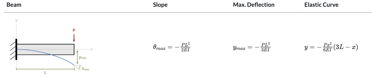
Beams are typically loaded in a relatively small number of standard configurations, and the deflection behavior of a beam subjected to one of these standard loads is very well understood. The slope and deflection equations for many common loading conditions have been derived through the methods described in Section 11.1 and Section 11.2 and recorded. A subset of these beam deflections has been included in Appendix B. Figure 11.8 shows an example of the information provided there for one such beam.

Figure 11.8: Appendix B contains some standard loading configurations along with a sketch of the elastic curve, equations for the maximum deflection and maximum slope, and the general equation of the elastic curve.

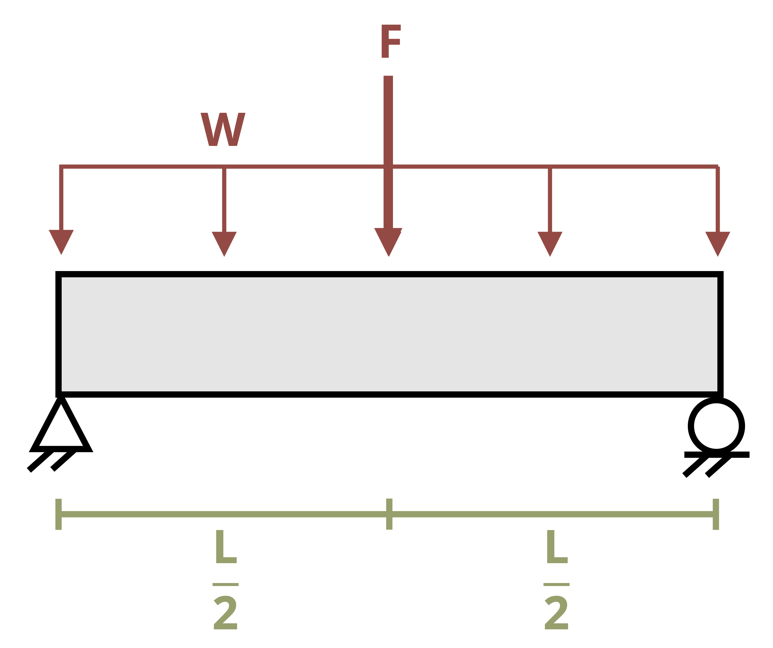
This information can be useful even for more complex loading. When multiple loads act on a beam, the effect of each load on the deflection of the beam may be considered independently. Thus even for loading more complex than the loads in Appendix B, it may be possible to simplify the problem by considering each load separately and calculating the deflection caused at a point by each load (Figure 11.9). These deflections can then be summed to find the overall deflection at that point. We must, of course, calculate the deflection at the same point for each load in order to add them together. See Example 11.5 for a demonstration.

Figure 11.9: Although Appendix B doesn’t contain a cantilever beam with both a distributed load and a concentrated load, it does contain cantilever beams with each load separately. We may find the combined deflection by finding the deflection of each load separately and adding them together.

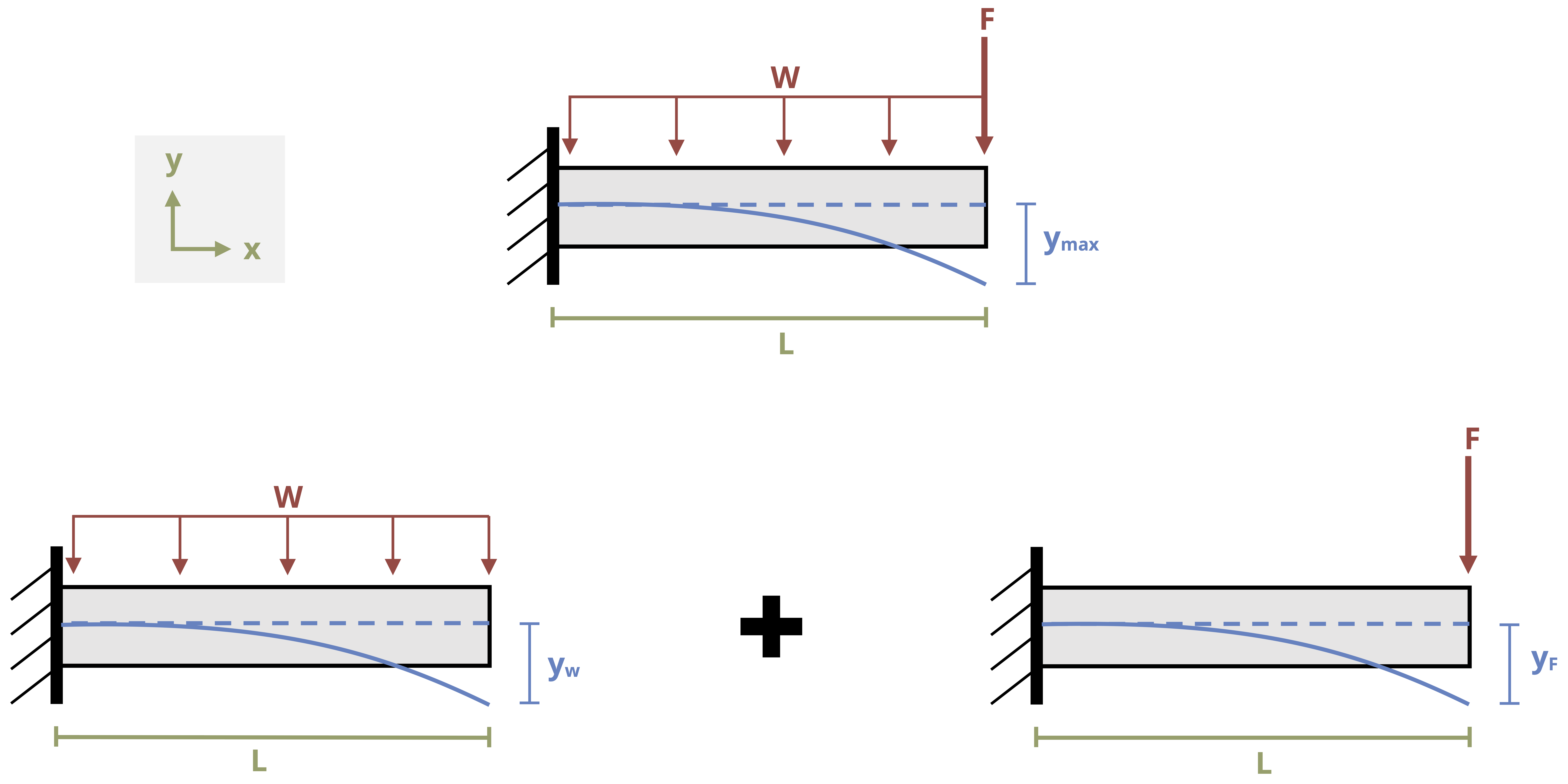
\[ \begin{aligned} y_w = - \frac{wL^4}{8EI} \quad \quad \quad \quad \quad \quad \quad \quad \quad \quad &\quad \quad \quad \quad \quad \quad \quad \quad \quad \quad y_F=-\frac{FL^3}{3EI} \\ y_{max}=-&\frac{wL^4}{8EI} - \frac{FL^3}{3EI} \end{aligned} \]

TipExample 11.5

Example 11.5  

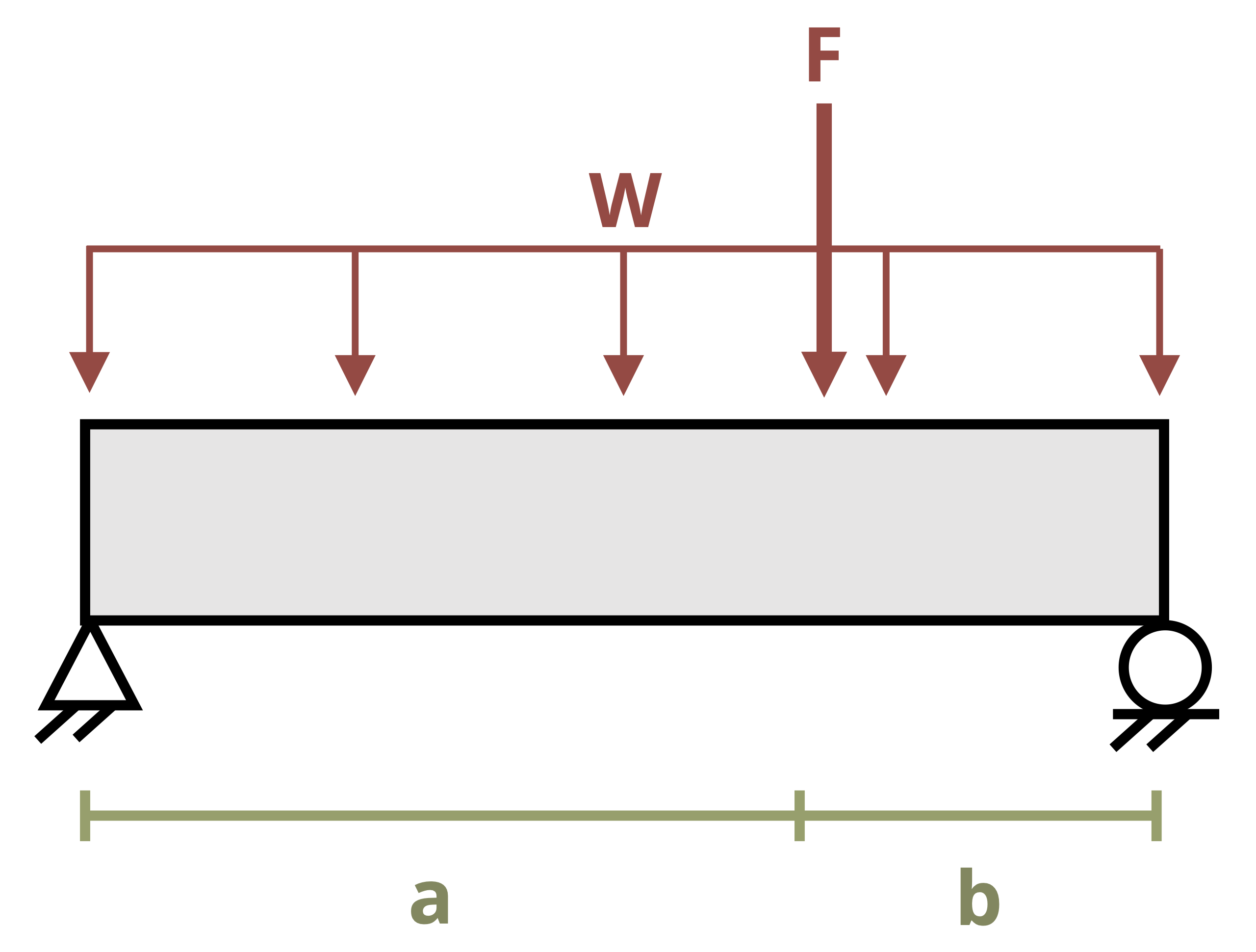
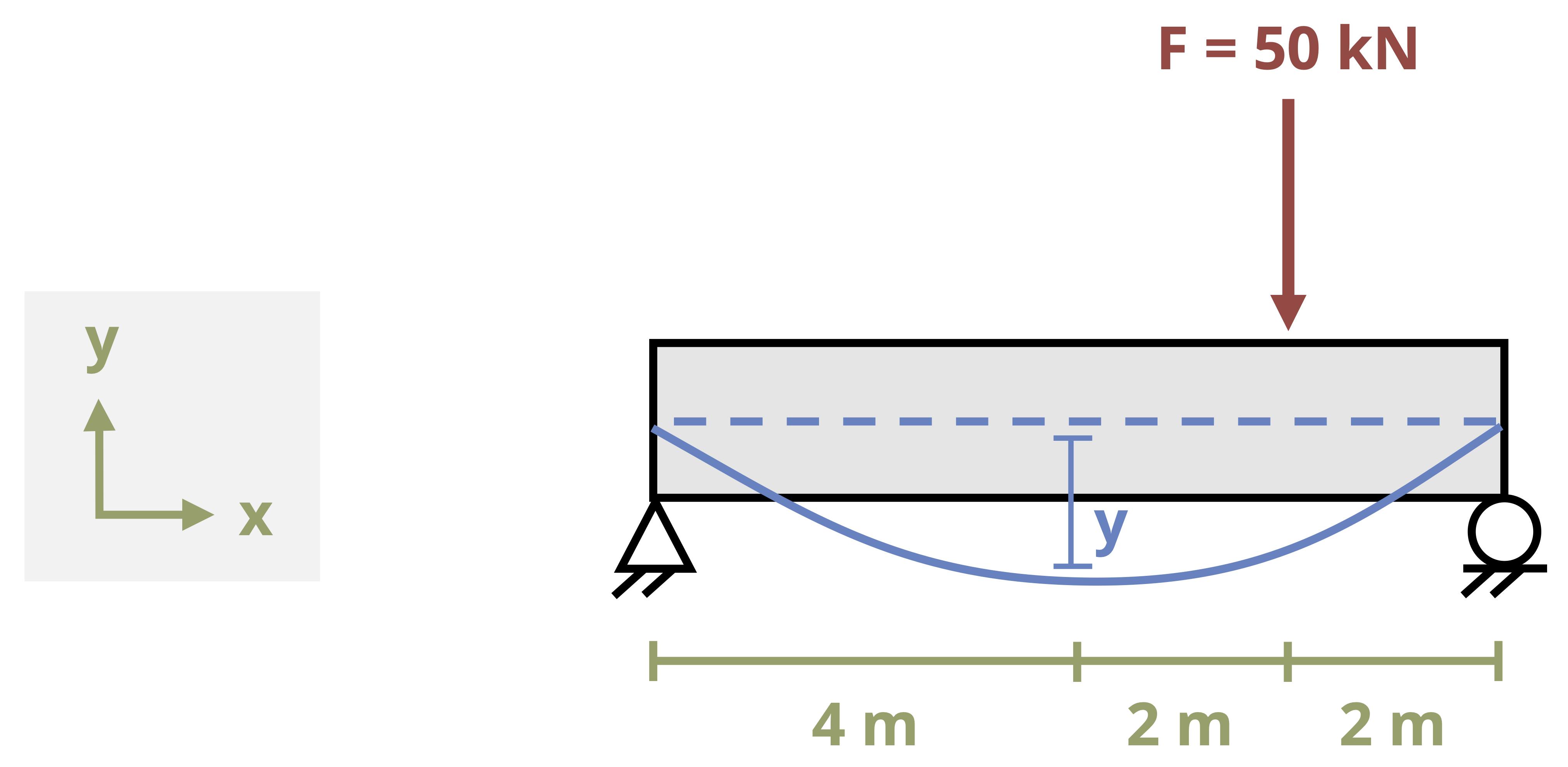
A simply supported beam is subjected to a distributed load w = 20 kN/m and a concentrated load F = 50 kN.

If distance a = 6 m and b = 2 m, determine the deflection at the midpoint of the beam (x = 4 m).

Assume E = 210 GPa and I = 275 x 10⁶ mm⁴.

TipSolution

Consider each load separately. We’ll start with the distributed load (although this step can be completed in any order).

Appendix B shows that the maximum deflection for this load occurs at the center of the beam, which is the point of interest.

\[ \begin{aligned} y&=-\frac{5 w L^4}{384EI} \\ &=-\frac{5*20,000~\frac{N}{m}*(8{~m})^4}{384*210 \times 10^9~\frac{N}{m^2} \times 275 \times 10^{-6}{~m}} \\ & =-0.01847{~m} \\ & =-18.47{~mm}\end{aligned} \]

Now consider the concentrated load.

Here the maximum deflection does not occur at the center of the beam. Use the elastic curve equation for x < a to find the deflection at x = 4 m when the load is applied at a = 6 m.

\[ \begin{aligned} y&=-\frac{Fbx}{6EIL}\left[L^2-b^2-x^2\right]\\ &=-\frac{50,000{~N}*2{~m}*4{~m}}{6*210 \times 10^9~\frac{N}{m^2}*275 \times 10^{-6}{~m^4}* 8{~m}}\left[(8~m)^2-(2~m)^2-(4~m)^2\right] \\ & =-~0.00635{~m} \\ & =-~6.35{~mm} \end{aligned} \]

The total deflection at the beam’s midpoint is

\[ \begin{aligned} & y=-~18.47{~mm}-6.35{~mm} \\ & y=-~24.8~mm \end{aligned} \]

WarningStep-by-Step: Deflection by Superposition

1. Sketch the beam with just one load acting on it.

2. Use Appendix B to find a beam with the same supports and loading.

3. Use the relevant equation in Appendix B to find the deflection at the point of interest.

4. Repeat this process until all loads have been considered. Add the individual deflections at the point of interest to find the overall deflection at this point.

11.4 Statically Indeterminate Deflection

Click to expand

A problem is statically indeterminate if there are more unknown support reactions than there are equilibrium equations to solve for them. These problems were introduced in Section 5.5 and Section 6.3. In both sections, to solve statically indeterminate problems we took advantage of our knowledge of deformation to solve for one of the reaction forces before using equilibrium equations to find the others. We’ll do something similar here. We may use either an integration method like that used in Section 11.1 or a superposition method like that used in Section 11.3.

In practice engineers design structures with redundancies so that if one part fails it can be replaced without the entire structure collapsing. As such, static indeterminacy is the norm.

In Section 11.1 we cut a cross-section and found the internal bending moment as a function of x, M = f(x). This was integrated twice to determine the equation of the elastic curve. For statically indeterminate problems, we’ll write the moment equation as a function of both x and A, where A is the unknown force at the redundant support. Integrating this equation twice results in three unknowns, but also three boundary conditions. These unknowns and boundary conditions enable us to solve for the redundant reaction force, and then we can use equilibrium equations to solve for the other reactions. See Example 11.6.

TipExample 11.6

Example 11.6  

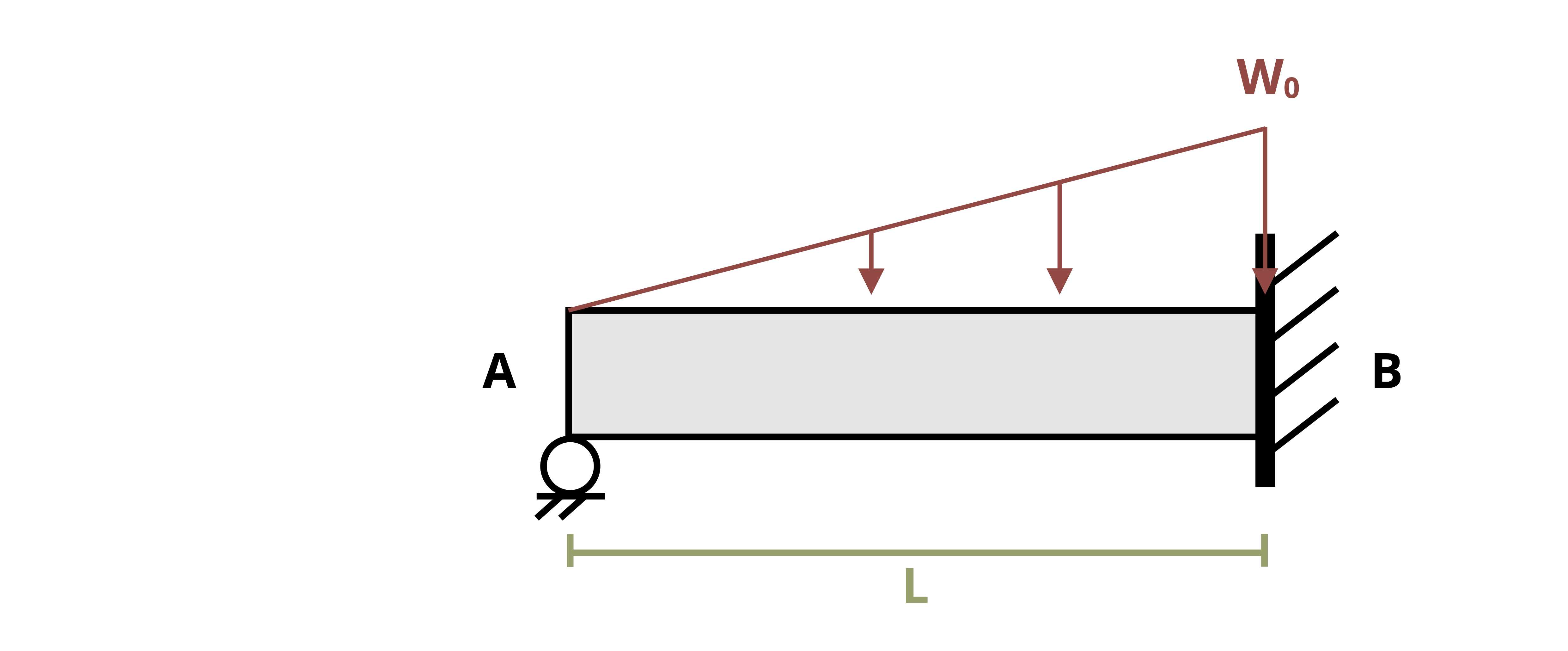
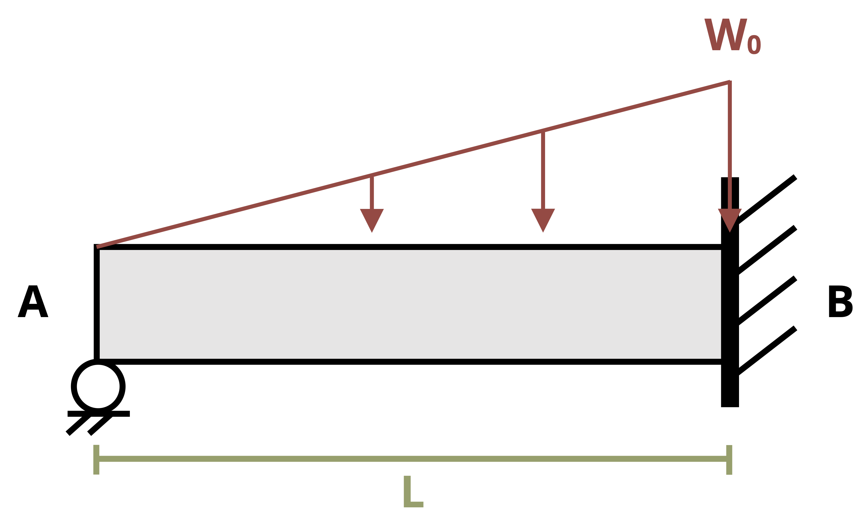
A propped cantilever beam of length L = 6 ft is subjected to a linear distributed load where w₀ = 20 kips/ft.

Determine the reactions at supports A and B.

TipSolution

An FBD of the beam shows four unknowns and only three equilibrium equations. We can solve \(\sum F_x=0\) to find \(B_x = 0\), but that still leaves us with three unknowns and two equations.

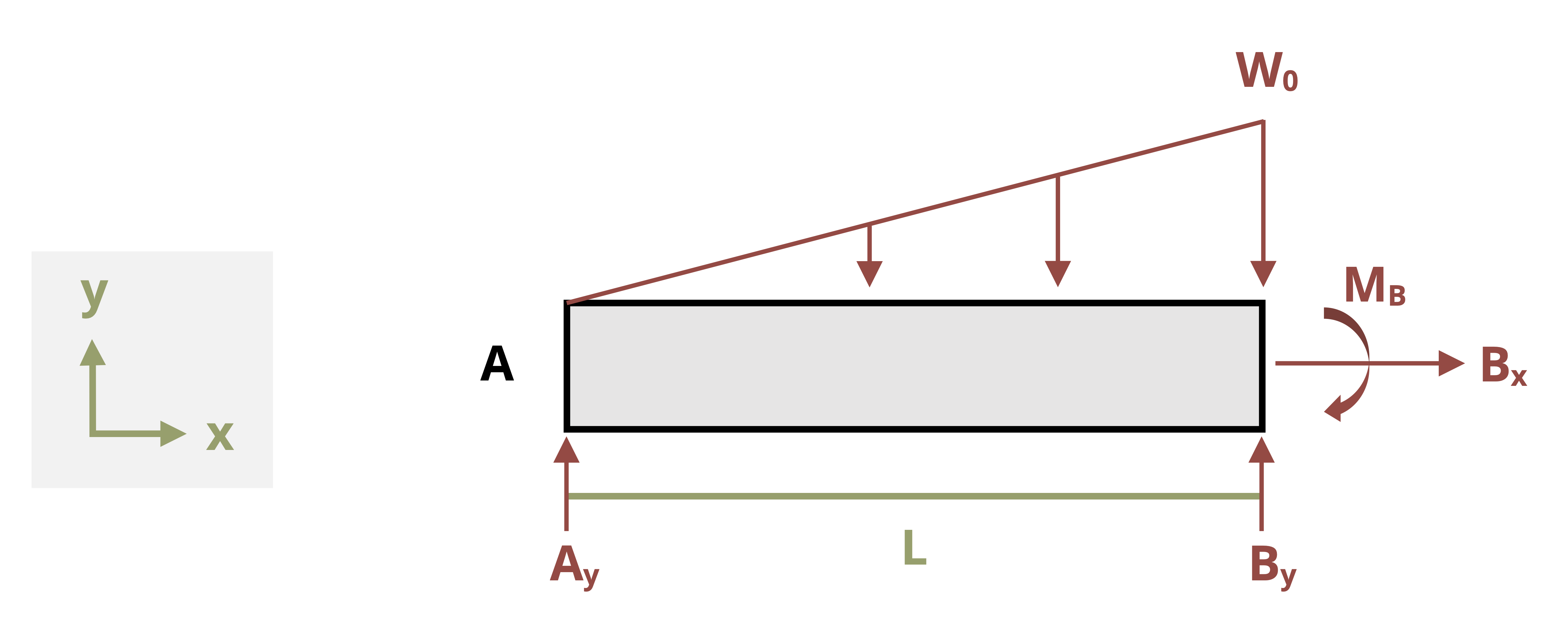
Cut a cross-section and determine the internal bending moment in terms of distance x and redundant force A_y. Set this equation equal to \(EI\frac{\partial^2 y}{\partial x^2}\) and integrate twice.

\[ \begin{aligned} \sum M_x=&~M+\frac{w_0 x^2}{2 L}\left(\frac{x}{3}\right)-A_y x=0 \\ M&=A_y x-\frac{w_0 x^3}{6 L}=EI \frac{\partial^2 y}{\partial x^2} \\ \int M~dx&=\frac{A_y x^2}{2}-\frac{w_0 x^4}{24 L}+c_1=E I \frac{\partial y}{\partial x} \\ \int\int M~dx&=\frac{A_y x^3}{6}-\frac{w_0 x^5}{120 L}+c_1 x+c_2=E I y\end{aligned} \]

Now we have three unknowns (A_y, c₁, c₂) and three boundary conditions (at the roller, deflection equals zero; at the fixed support, both slope and deflection equal zero).

Apply the boundary conditions.

\[ \begin{aligned} & \text { At } x=0, y=0 \quad \rightarrow \quad c_2=0 \\ & \text { At } x=L, y=0 \quad \rightarrow \quad \frac{A_y L^3}{6}-\frac{w_0 L^4}{120}+c_1 L=0 \\ & \text { At } x=L, \frac{\partial y}{\partial x}=0 \quad \rightarrow \quad \frac{A y L^2}{2}-\frac{w_0 L^3}{24}+c_1=0\end{aligned} \]

Rearrange and substitute.

\[ \begin{gathered}c_1=\frac{w_{0 L}{ }^3}{24}-\frac{A_y L^2}{2} \\ \frac{A_y L^3}{6}-\frac{w_0 L^4}{120}+\frac{w_0 L^4}{24}-\frac{A_y L^3}{2}=0 \\ \frac{-2 A_y L^3}{6}+\frac{4 w_{0} L^4}{120}=0 \\ A_y=\frac{w_0 L}{10}\end{gathered} \]

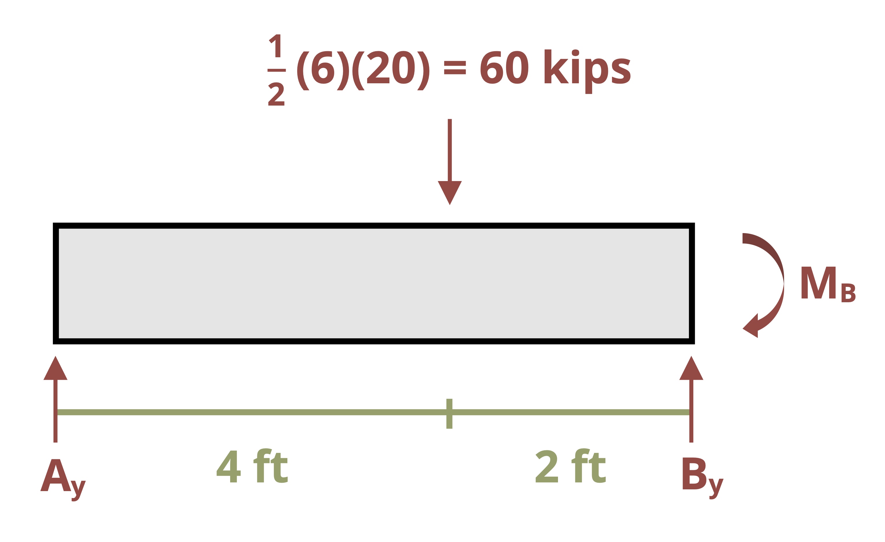
We can now reach a numerical answer and find the other reactions by equilibrium.

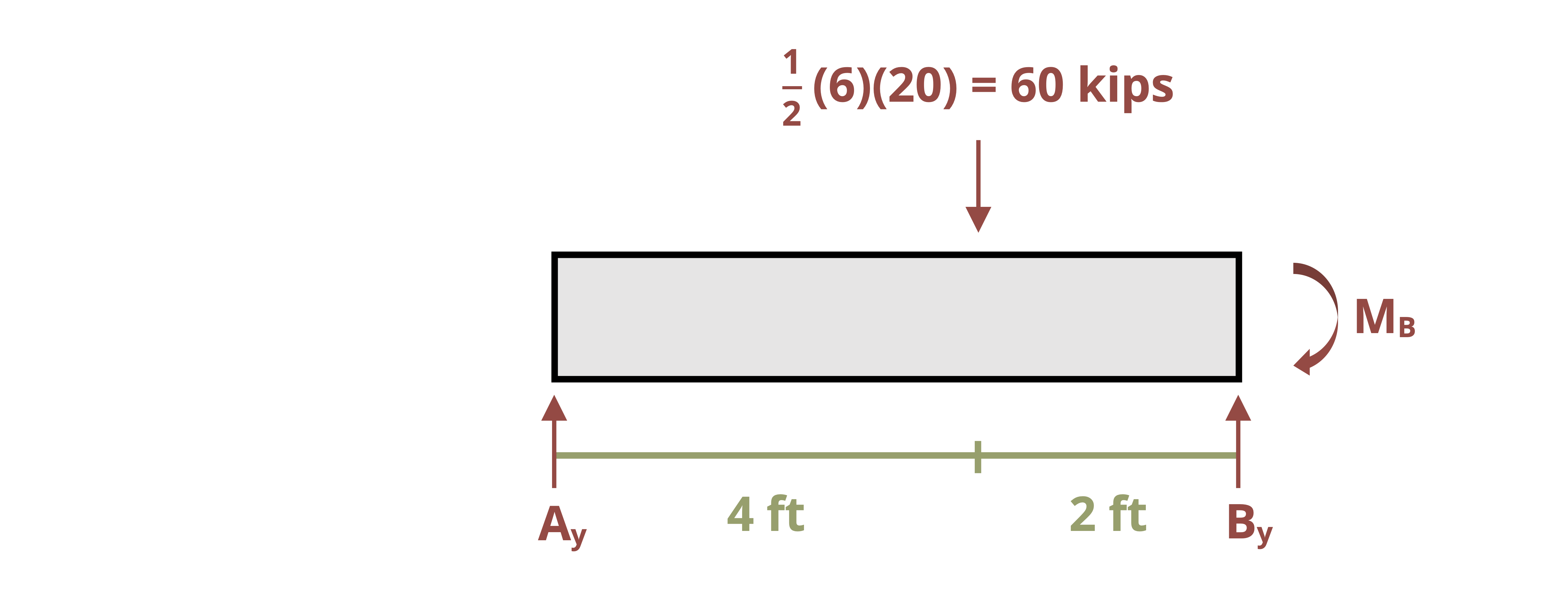
\[ \begin{aligned} &A_y=\frac{20~\frac{kips}{ft}*6{~ft}}{10}=12{~kips} \\ \\ & \sum F_y=12{~kips}-60{~kips}+B_y=0 \quad \rightarrow \quad B_y=48{~kips} \\ & \sum M_A=-(60{~kips}* 4{~ft})+(48{~kips}*6{~ft})-M_B=0 \quad \rightarrow \quad M_B=48{~kip}\cdot{ft} \\ & \end{aligned} \]

This method works well for beams with a single continuous load. While it can be used for more complex loads, it quickly becomes complicated and time-consuming. For these cases superposition is recommended.

The superposition method is like the methods used to solve other statically indeterminate problems in Section 5.5 and Section 6.3. To solve a statically indeterminate deflection problem using superposition, first identify the redundant support. We have three equilibrium equations and so can solve for three unknown support reactions. Any support reactions beyond these three are redundant.

Remove each redundant reaction and determine the deflection resulting from the applied loads at the point where the reaction was removed. Without fail do this for each redundant reaction. It is best to remove a support such that the remaining beam is either simply supported or cantilever, given that these are the only support configuration in Appendix B.

Then replace each redundant reaction and determine the resulting deflection where the reaction is applied. Since there is actually a support here, the total deflection must be zero. Sum both deflections and set them equal to zero. This enables you to calculate the value of the redundant support. Once this is known, the other reaction loads can be determined using equilibrium. See Example 11.7 for a demonstration.

TipExample 11.7

Example 11.7  

The propped cantilever beam of Example 11.6 is shown again here. Length L = 6 ft and is subjected to a linear distributed load where w₀ = 20 kips/ft.

Determine the reactions at supports A and B.

TipSolution

As demonstrated in Example 11.6, this problem is statically indeterminate.

This time remove redundant support A_y and use Appendix B to find the deflection at point A.

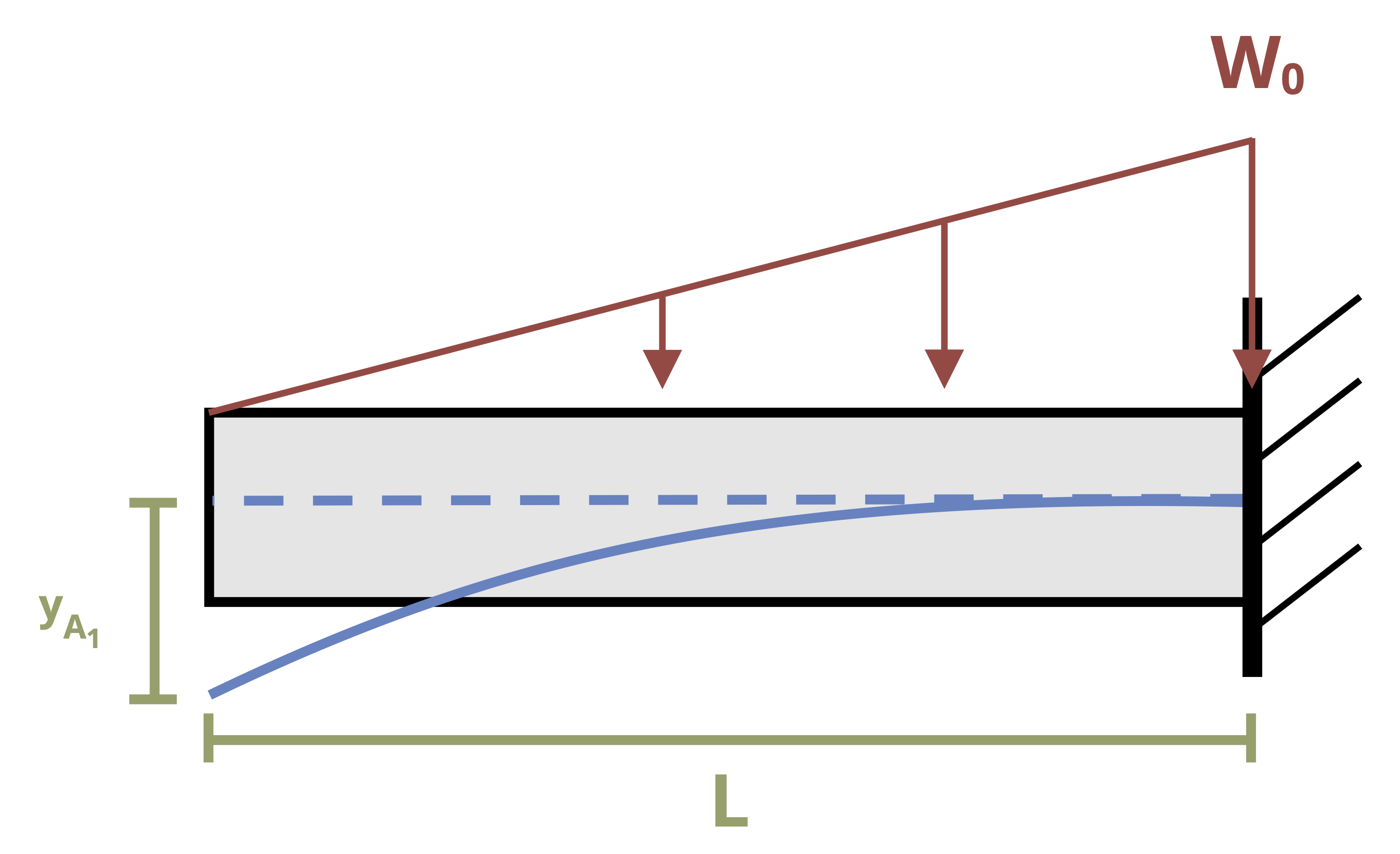
\[ y_{A_1}=-\frac{w_0 L^4}{30 E I} \]

Now replace A_y and use Appendix B to find the deflection at point A caused by A_y.

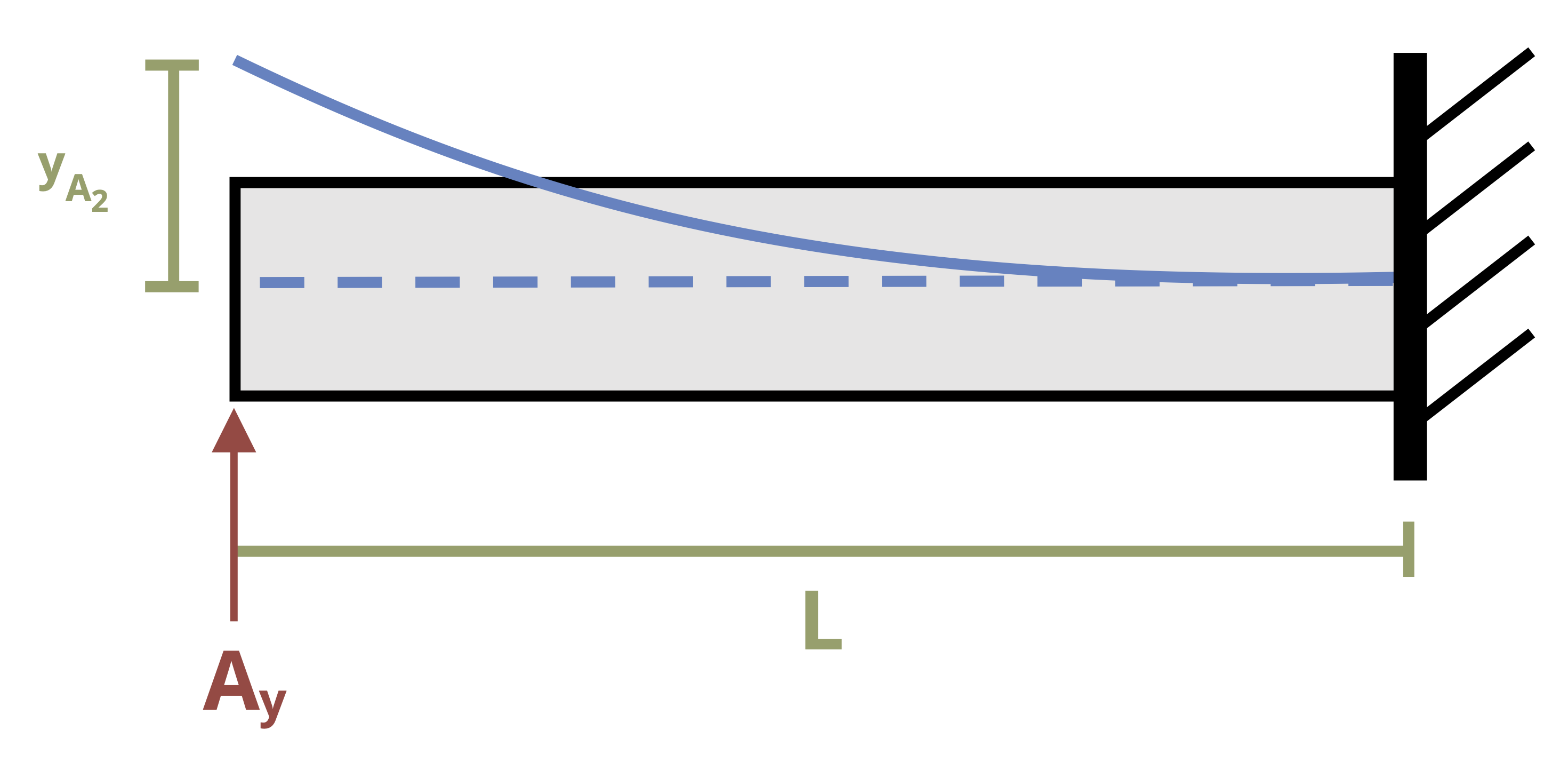
\[ y_{A_2}=\frac{A_{y L}{ }^3}{3 E I} \]

Since there is actually a support at A, the deflection at A must be zero.

\[ -\frac{w_0 L^4}{30 E I}+\frac{A_y L^3}{3EI}=0 \quad \rightarrow \quad A_y=\frac{W_0 L}{10} \]

This is the same answer found in Example 11.6, and the rest of the problem proceeds in the same way.

\[ \begin{aligned} &A_y=\frac{20~\frac{kips}{ft}*6{~ft}}{10}=12{~kips} \\ \\ & \sum F_y=12{~kips}-60{~kips}+B_y=0 \quad \rightarrow \quad B y=48{~kips} \\ & \sum M_A=(60{~kips}* 4{~ft})+(48{~kips}*6{~ft})-M_B=0 \quad \rightarrow \quad M_B=48{~kip}\cdot{ft} \\ & \end{aligned} \]

It’s possible to remove a moment reaction so that what remains is a simply supported beam. In this case, determining the deflection at the point where the load was removed isn’t helpful because removing the moment reaction from a fixed support effectively leaves a pin support and the deflection with the moment removed will still be zero. In this situation look at the slope at the point where the reaction was removed.

Example 11.7 is repeated with the moment at B removed instead of the force at A.

TipExample 11.7 (reworked)

The propped cantilever beam of Example 11.6 is shown again here. Length L = 6 ft is subjected to a linear distributed load where w₀ = 20 kips/ft.

Determine the reactions at supports A and B.

TipSolution

This time remove the moment reaction at B to leave a simply supported beam.

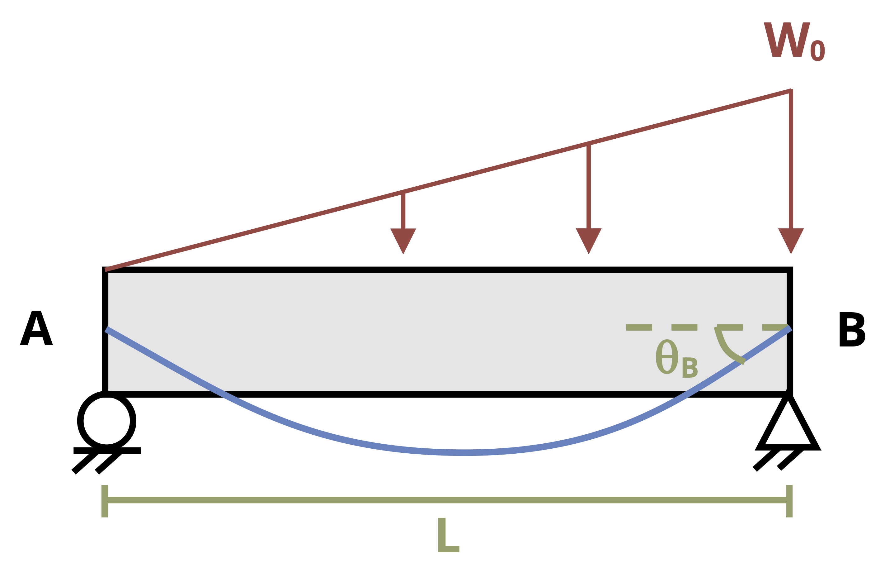
Finding the deflection at B would not help as it would simply be zero. Instead, use Appendix B to find the slope at B.

\[ \theta_B=\frac{W_0 L^3}{45 E I} \]

Now replace the moment reaction at B and use Appendix B to find the slope at B due to this moment.

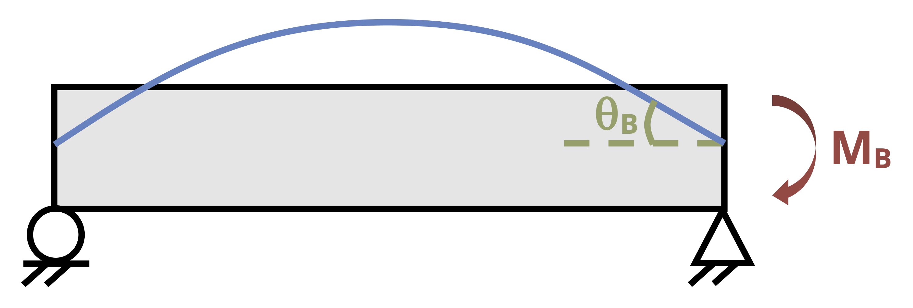
\[ \theta_B=-\frac{M_B L}{3 E I} \]

Since there is actually a fixed support at B, the slope here must be zero.

\[ \begin{aligned} &\frac{W_0 L^3}{45 E I}-\frac{M_{B L}}{3 E I}=0 \\ &M_B =\frac{W_0 L^2}{15}\end{aligned} \]

Adding numbers yields

\[ M_B=\frac{20~\frac{kips}{ft}*(6{~ft})^2}{15}=48{~kip}\cdot{ft} \]

This is the same answer found in Example 11.6. Reactions A_y and B_y can be found by equilibrium and will also result in the same answers as in Example 11.6.

\[ \begin{aligned} &\sum M_A=(60{~kips}*4{~ft})+48{~kip}\cdot{ft}-(B_y*6{~ft})=0 \quad\rightarrow\quad B_y=48{~kips} \\ &\sum F_y=A_y+-60{~kips}+48{~kips}=0 \quad\rightarrow\quad A_y=12{~kips}\\ \end{aligned} \]

Note that some problems may involve multiple redundant reactions. In such cases remove all redundant reactions and determine the deflection from the external loads at every point where a reaction was removed. Then replace the redundant reactions one at a time and determine the deflection from each load at every point where a reaction was removed. As before, the total deflection at each of these points must be zero. Sum the deflection at each point and set it equal to zero. There will be one equation for every redundant reaction, and so all redundant reactions can be calculated.

WarningStep-by-Step: Statically Indeterminate Deflection

1. Identify and remove redundant reaction(s).

2. Determine the deflection at the point where the reaction was removed. Use superposition if possible, or integration otherwise.

   • If the removed reaction was a moment, determine the slope at this point instead.

3. Replace the redundant reaction and determine the deflection caused by this load at the point where the load acts.

   • If the removed reaction was a moment, determine the slope at this point instead.

4. These deflections (or slopes) must add up to the total deflection at this point. This is typically zero due to the support unless indicated otherwise. Use this to determine the magnitude of the redundant reaction.

5. Use equilibrium to solve for the other reactions. Then solve for anything else required as normal.

11.5 Beam Design for Bending, Shear, and Deflection

Click to expand

Section 9.2 showed us how to use the section modulus to design a beam to meet bending stress specifications. In practice, beams must also meet specifications for shear stress and deflection. Limitations are placed on all three of these criteria, and we must design our beams to meet all three simultaneously. We’ll begin with rectangular cross-sections and then move on to standard beams using Appendix A.

As in Section 9.2, problems involving rectangular cross-sections typically relate the base and height of the cross-section such that only one dimension must be determined. Previously we designed the cross-section to resist bending stress using

\[ S_{\min }=\frac{M_{\max }}{\sigma_{allow}}=\frac{I}{c} \]

Since \(I=\frac{b h^{3}}{12}\) and \(c=\frac{h}{2}\), we were able to determine the required dimensions to meet the minimum required section modulus. Note that the equation \(S=\frac{I}{c}\) simplifies to \(S=\frac{\frac{b h^{3}}{12}}{\frac{h}{2}}=\frac{2 b h^{3}}{12 h}=\frac{b h^{2}}{6}\) for a rectangle.

To meet the minimum required shear stress, use \(\tau=\frac{V Q}{I t}\). Applying the method of Section 10.1, to a rectangle (Figure 11.10) shows that \(Q=y A=\frac{h}{4} \frac{b h}{2}=\frac{b h^{2}}{8}\).

With \(I=\frac{b h^{3}}{12}\) and \(\mathrm{t}=\mathrm{b}\), rewrite the shear stress equation to find the maximum shear stress in a rectangular cross-section as \(\tau_{\max }=\frac{V \frac{b h^{2}}{8}}{\frac{b h^{3}}{12} b}=\frac{12 V b h^{2}}{8 b^{2} h^{3}}=\frac{12 V}{8 b h}=\frac{3}{2} \frac{V}{A}\).

Figure 11.10: Rectangular cross-section showing the dimensions used for calculating the section modulus (S) and first moment of area (Q)

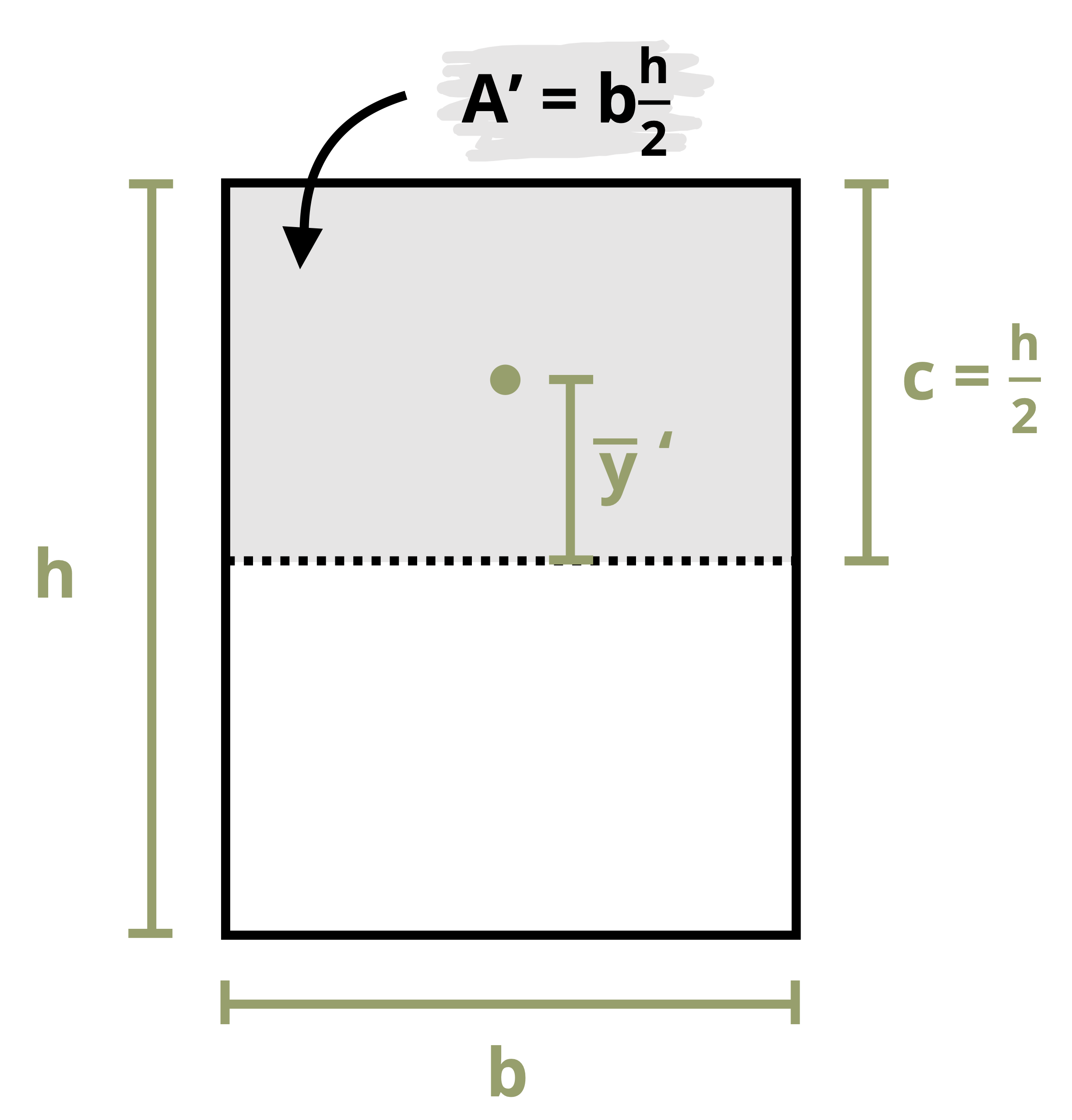
Thus set \(\tau_{\max }=\frac{3}{2} \frac{V}{A}\) and solve for the required dimensions to not exceed the maximum allowable shear stress.

The maximum deflection of the beam under a given loading configuration can be found using the methods shown in this chapter. Wherever possible use superposition and Appendix B. If it’s not possible to do so, then use the method of integration instead. In either case the equation for the beam’s maximum deflection will include the second moment of area, I. Set the maximum allowable deflection equal to this equation and replace \(I=\frac{b h^{3}}{12}\).

Then solve for the cross-section’s required dimensions to not exceed the maximum allowable deflection of the beam.

You now have three different dimensions: one required to not exceed the maximum bending stress, one required to not exceed the maximum shear stress, and one required to not exceed the maximum deflection. Since none of these limitations may be exceeded, select the largest of the three potential answers. See Example 11.8 for a demonstration.

TipExample 11.8

Example 11.8  

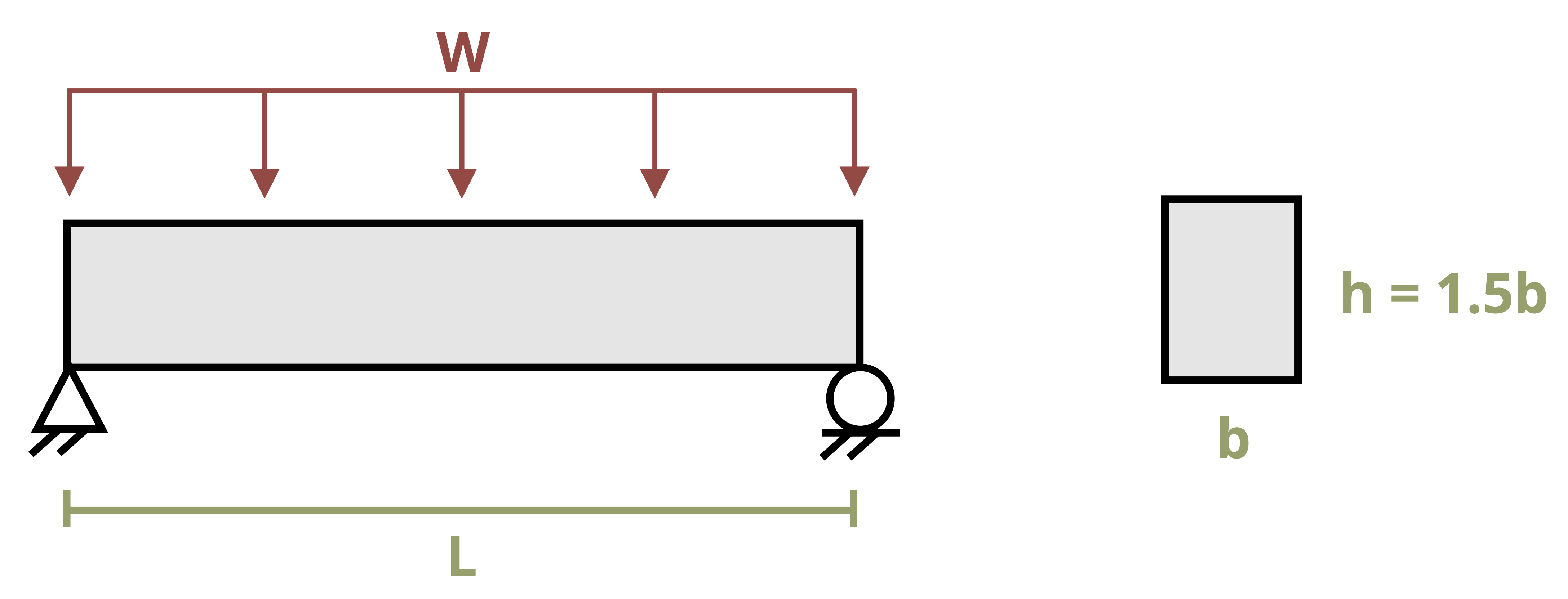
The simply supported wooden beam (E = 1,700 ksi) of length L = 12 ft is subjected to a uniform distributed load of w = 1.5 kips/ft.

Assume the beam has an allowable bending stress of 900 psi, an allowable shear stress of 180 psi, and a deflection limited to beam span / 240.

The beam has a rectangular cross-section where h = 1.5b.

Determine the minimum required dimensions of the beam’s cross-section to meet these specifications. Give your answer rounded up to the nearest inch to allow for realistic manufacturing tolerances.

TipSolution

Start by drawing shear force and bending moment diagrams to determine the maximum internal loads.

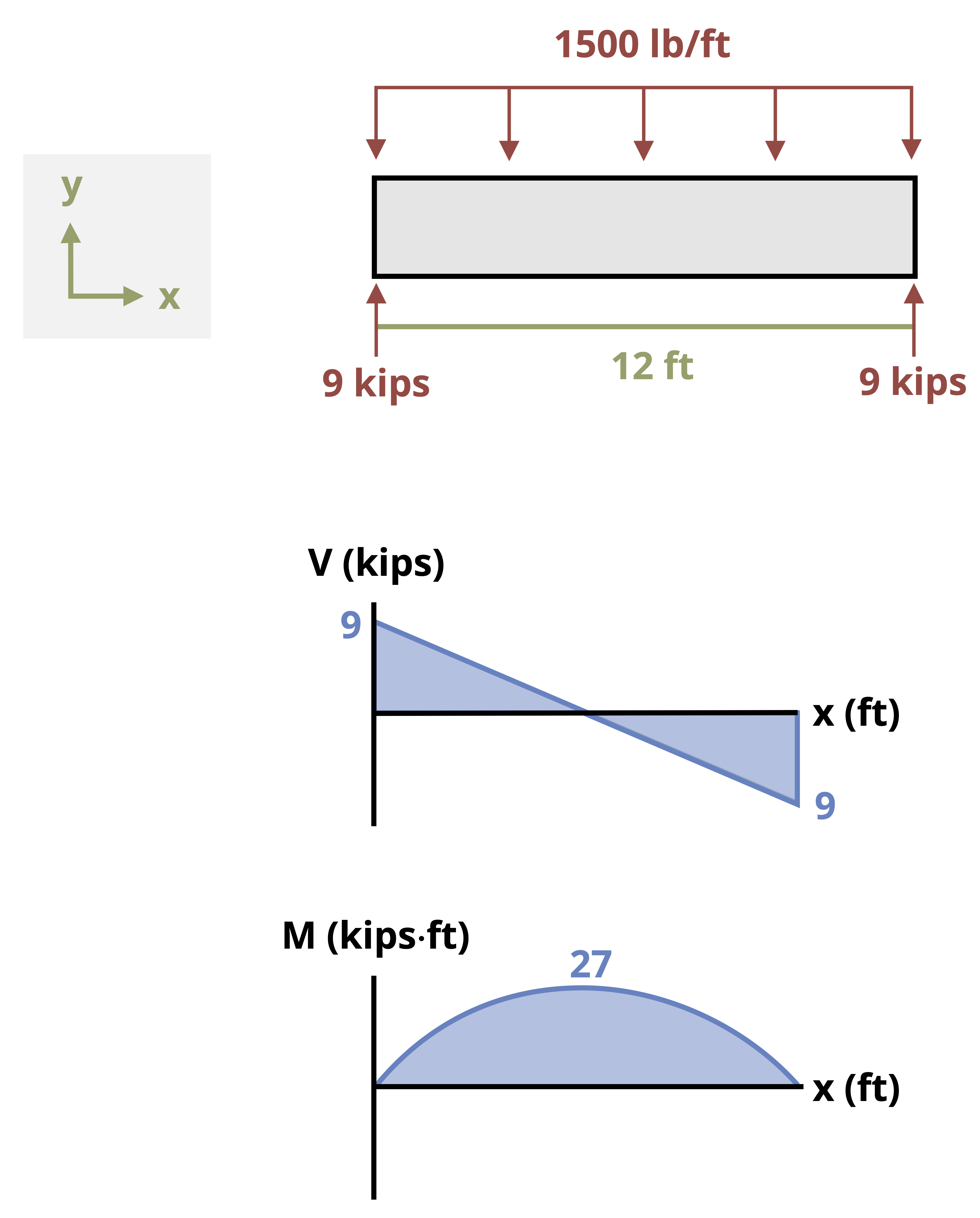
V_max = 9 kips

M_max = 27 kip·ft

Design for bending by using the minimum required section modulus, S_min.

\[ \begin{aligned} & S_{min}=\frac{M_{max}}{\sigma_{allow}}=\frac{27,000{~lb}\cdot{ft}*12~\frac{in.}{ft}}{900~\frac{lb}{in.^2}}=360{~in.^3} \\ & 360{~in.^3}=\frac{b h^2}{6}=\frac{b(1.5b)^2}{6}=\frac{2.25 \mathrm{~b}^3}{6} \\ & b =9.865{~in.} \end{aligned} \]

Design for shear.

\[ \begin{aligned} & \tau_{max}=\frac{3}{2} \frac{V}{A} \\ & 180~\frac{lb}{in.^2}=\frac{3}{2}*\frac{9,000{~lb}}{A} \\ & A=\frac{3}{2}*\frac{9,000{~lb}}{180~\frac{lb}{in.^2}}=75{~in.^2} \\ & 75{~in.^2}=b h=b(1.5 b)=1.5 b^2 \\ & b=7.071{~in.} \end{aligned} \]

Design for deflection.

From Appendix B note that

\[ y_{\max }=- \frac{5 w L^4}{384 E I} \]

\[ \begin{gathered} -\frac{Span}{240}=-\frac{(12{~ft}*12~\frac{in.}{ft})}{240}=-\frac{5*\frac{1,500~\frac{lb}{ft}}{12~\frac{in.}{ft}}*(12{~ft}*12\frac{in.}{ft})^4}{384*1,700,000~\frac{lb}{in.^2}*I} \\ I=\frac{bh^3}{12}=\frac{b(1.5b)^3}{12}=\frac{3.375b^4}{12}=\frac{5*\frac{1,500~\frac{lb}{ft}}{12\frac{in.}{ft}}+(12{~ft}*12\frac{in.}{ft})^4}{384*1,700,000~\frac{lb}{in.^2}}*\frac{240}{\left(12{~ft}*12\frac{in.}{ft}\right)} \\ b=7.028{~in.} \end{gathered} \]

Select the largest dimension required to meet all these criteria.

\[ b_{req}=9.865{~in.} \\ h_{req}=1.5b_{req}=14.8{~in.} \]

Calculate to the next nearest inch.

\[ \begin{aligned} & b_{req}=10 \mathrm{~in.} \\ & h_{req}=15{~in.}\end{aligned} \]

For standard beams again use the method of Section 9.2 to select a beam from Appendix A that meets the specifications for bending stress. Use \(S_{\min }=\frac{M_{\max }}{\sigma_{allow}}\) and select a beam with \(\mathrm{S}>\mathrm{S}_{\min }\).

Next determine the equation for the beam’s maximum deflection under the given loading conditions. As before, use superposition and Appendix B whenever possible. Set the maximum allowable deflection equal to this equation and solve for the minimum required second moment of area, \(I_{\min }\). Now select the lightest beam from Appendix A that meets both \(S_{\min }\) and \(I_{\min }\).

Steel W beams rarely fail from shear stress, but shear must nonetheless be checked. An exact value for the maximum shear stress in the beam can be found from \(\tau_{\max }=\frac{V Q}{I t}\). However, the beam’s web resists most of the shear stress. A reasonable estimate of the maximum shear stress can be found using \(\tau_{estimate}=\frac{V}{A_{web}}\). This calculation is relatively simple, but it’s important to note that it is only an estimate. In most cases the maximum shear stress will be significantly less than the allowable shear stress, and this estimate will suffice to demonstrate that. In the rare case that the maximum shear stress is within 20 percent of the allowable shear stress, an exact value must be determined using \(\tau_{\max }=\frac{V Q}{I t}\).

The beam was selected to meet the bending stress and deflection requirements. As long as the maximum shear stress is less than the allowable shear stress, the beam can be used. See Example 11.9 for a demonstration.

TipExample 11.9

Example 11.9  

A steel (E = 210 GPa) W-beam of length L = 10 m needs to support the load shown, where w = 5 kN/m and F = 100 kN.

Assume the beam has an allowable bending stress of 150 MPa, an allowable shear stress of 100 MPa, and a maximum deflection limited to 40 mm.

Select the lightest weight W-beam from Appendix A that meets these specifications.

TipSolution

Load is symmetric, so each support will hold half the load. Draw shear force and bending moment diagrams to find the maximum internal loads.

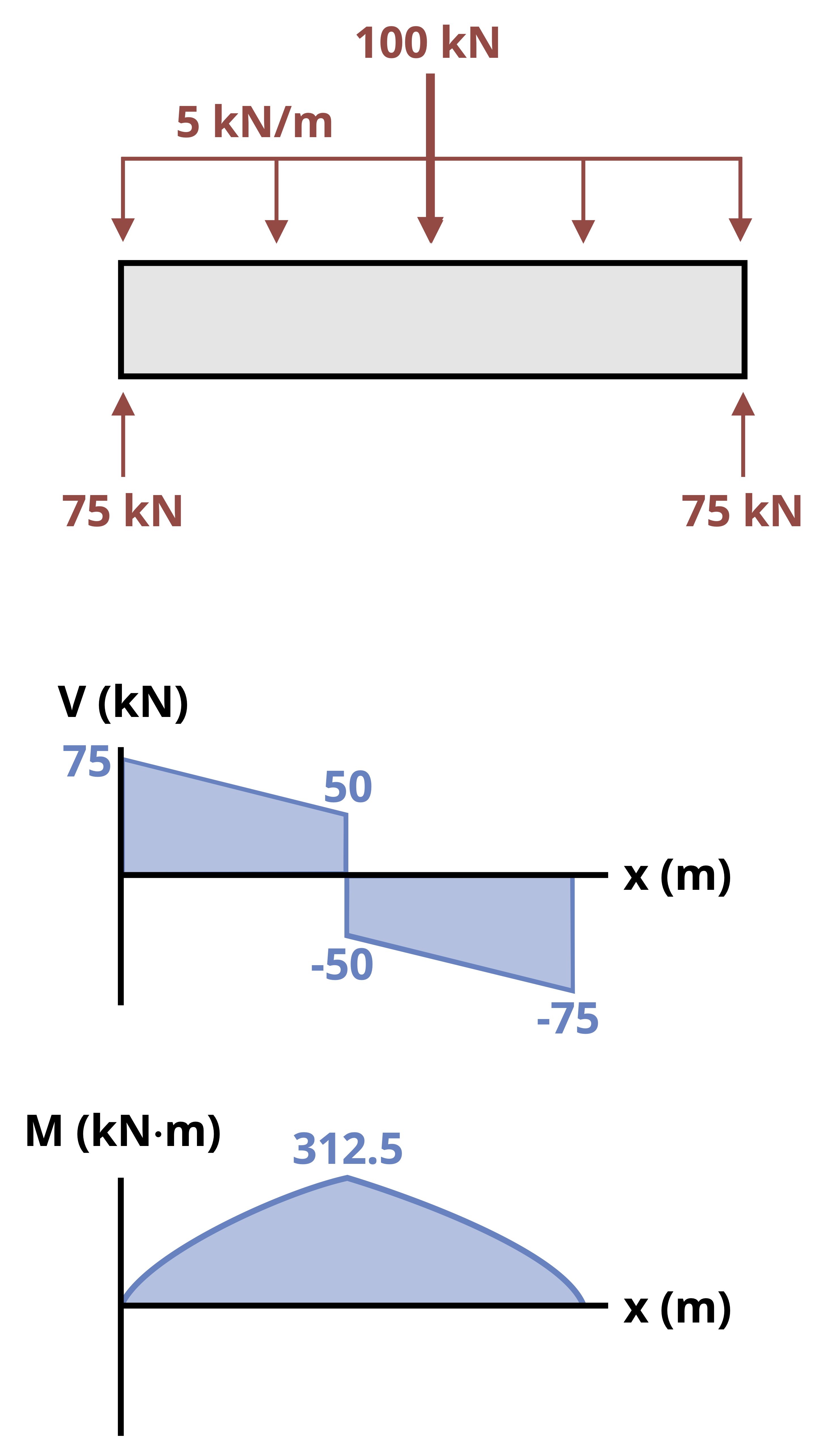
V_max = 75 kN

M_max = 312.5 kN·m

Design for bending by using the minimum required section modulus S_min.

\[ \begin{aligned} S_{min}=\frac{M_{max}}{\sigma_{Allow}}=\frac{312.5\times10^3{~N}\cdot{m}}{150 \times 10^6~\frac{N}{m^2}} & =0.002083{~m}^3 \\ & =2,083 \times 10^3{~mm}^3 \\ \end{aligned} \]

Design for deflection.

We know the maximum deflection is limited to 40 mm (0.04 m) and the beam will deflect downward. From Appendix B we can see the maximum deflection for both the concentrated load and the distributed load occur in the same place. We can therefore add the two maximum deflection equations together and solve for the second moment of area.

\[ \begin{aligned} y_{max}&= -0.04{~m}=-\frac{5wL^4}{384EI}-\frac{FL^3}{48EI} \\ I_{req}&=\frac{1}{0.04{~m}}\left[\frac{5*5,000~\frac{N}{m}*(10{~m})^4}{384*(210 \times 10^9)~\frac{N}{m^2}}+\frac{100,000{~N}*(10{~m})^3}{48*(210 \times 10^9)~\frac{N}{m^2}}\right] \\ I_{req}&=0.0003255{~m}^4 \\ &= 325.5 \times 10^6{~mm}^4 \end{aligned} \]

Select the lightest beam from Appendix A with

\[ \begin{aligned} & S>2,083\times10^3{~mm}^3 \\ & I>325.5\times10^6 {~mm}^4 \end{aligned} \]

Options include

\[ \begin{aligned}&W310\times158\quad(S=2380\times10^3~mm^3,I=388\times10^6~mm^4)\\ &W360\times134\quad(S=2,340\times10^3~mm^3,I=416\times10^6~mm^4)\\ &W460\times113\quad(S=2,390\times10^3~mm^3,I=554\times10^6~mm^4)\\ &W530\times101\quad(S=2,290\times10^3~mm^3,I=616\times10^6~mm^4)\\ &W610\times125\quad(S=3,210\times10^3~mm^3,I=986\times10^6~mm^4)\\ &W760\times147\quad(S=4,410\times10^3~mm^3,I=1,660\times10^6~mm^4)\\ \end{aligned} \]

Select the lightest of these beams.

Use W530 x 101.

Check the estimated shear stress to ensure there’s no risk of exceeding the allowable shear stress.

\[ \begin{aligned} {\text{For }}W530\times 101, A_{web}&=t_w d \\ &=0.01098{~m}*0.536{~m} \\ &=0.0058853{~m}^2 \\ \tau=\frac{v_{max}}{A_{web}}=\frac{75,000{~N}}{0.0058853{~m^2}}&=12.7{~MPa} \end{aligned} \]

Since \(\tau_{Allow}=100 ~MPa\), this will be fine. The estimated shear stress is not close to the allowable shear stress.

WarningStep-by-Step: Intermediate Beam Design

Rectangular cross-sections:

1. Determine minimum required section modulus, \(S_{\min }=\frac{M_{\max }}{\sigma_{allow}}=\frac{b h^{2}}{6}\) and determine the minimum dimensions to meet the required \(\mathrm{S}_{\mathrm{min}}\).

2. Set the maximum allowable shear stress, \(\tau_{\max }=\frac{3}{2} \frac{\mathrm{V}}{\mathrm{A}}\), and determine the minimum dimensions to not exceed \(\tau_{\max }\).

3. Determine the maximum deflection for the applied load(s) and set this equal to the maximum allowable deflection. This equation will contain I, which depends on dimensions b and h. Determine the minimum dimensions to not exceed the maximum allowable deflection.

4. Use the largest of the three calculated dimensions, given that these will be the smallest dimensions that meet all three requirements.

Standard beams:

1. Determine minimum required section modulus, \(S_{\min }=\frac{M_{\max }}{\sigma_{allow}}\).

2. Determine the maximum deflection for the applied load(s) and set this equal to the maximum allowable deflection. Determine the minimum required second moment of area, \(I_{\min }\), to not exceed the maximum allowable deflection.

3. Select the lightest beam from Appendix A that meets both the \(S_{\min }\) and the \(I_{\min }\) requirements.

4. Estimate the maximum shear stress in the selected beam using \(\tau=\frac{V}{A_{w e b}}\). If this is within approximately 20 percent of the maximum allowable shear stress, calculate the maximum shear stress using \(\tau_{\max }=\frac{V Q}{I t}\).

5. If the maximum shear stress is less than the maximum allowable value, use this beam. If it’s greater than the maximum allowable value, return to step 3 and select the next lightest beam that meets both the \(S_{\min }\) and \(I_{\min }\) requirements.

Summary

Click to expand

NoteKey Takeaways

• Beams under load will experience a type of deformation known as deflection. It is typically required to limit deflection to some small amount.

• Deflection can be determined using either the method of integration or the method of superposition.

• Both methods can be used for both statically determinate and statically indeterminate beams, though superposition is recommended whenever possible as it is generally quicker than integration.

• Engineers designing beams must consider the response of the beam to bending stress, shear stress, and deflection simultaneously.

NoteKey Equations

Deflection by integration:

\[ \begin{aligned} &w(x)=E I \frac{d^{4} y}{d x^{4}} \\ &V(x)=E I \frac{d^{3} y}{d x^{3}}=\int w(x) d x+C 1 \\ &M(x)=E I \frac{d^{2} y}{d x^{2}}=\int V(x) d x+C 2 \\ &\theta(x)=E I \frac{d y}{d x}=\int M(x) d x+C 3 \\ &y(x)=\int \theta(x) d x+C 4 \end{aligned} \]

Boundary conditions:

• At any support the deflection is 0.

• At a fixed support both the slope and deflection are zero.

• The shear force will be equal to the applied force (including a force applied by a support) if there is one, or zero otherwise.

• The bending moment will be equal to the applied moment (including a moment applied by a fixed support) if there is one, or zero otherwise.

Beam design for rectangular cross-sections:

\[ \begin{gathered} S=\frac{b h^{2}}{6} \\ \tau_{\max }=\frac{3}{2} \frac{V}{A} \end{gathered} \]

Beam design for W beams:

\[ \begin{gathered} S_{min}=\frac{M_{max}}{\sigma_{allow}} \\ \tau_{max}=\frac{V Q}{I t} \\ \tau_{estimate} =\frac{V}{A_{web}} \end{gathered} \]

References

Click to expand

Figures

All figures in this chapter were created by Kindred Grey in 2025 and released under a CC BY license, except for

• Figure 11.1: A model bridge showing severe deflection along its span (left). Left: Denise Krebs. 2012. CC BY. https://flic.kr/p/bnc8qp. Right: clyde. 2012. CC BY-NC. https://flic.kr/p/bpkcyR.